Download
1 / 55
550 likes | 575 Views
Learn about the limitations of regular languages, parser overview, CFGs, syntax-directed translation, and the functionality of parsers. Explore the importance of formal languages in computer science. Programming language structure and notation are also discussed. Discover how context-free grammars play a crucial role in defining programming languages.

E N D
Introduction to Parsing Lecture 8 Adapted from slides by G. Necula and R. Bodik Prof. Hilfinger CS164 Lecture 8
Outline • Limitations of regular languages • Parser overview • Context-free grammars (CFG’s) • Derivations • Syntax-Directed Translation Prof. Hilfinger CS164 Lecture 8
Languages and Automata • Formal languages are very important in CS • Especially in programming languages • Regular languages • The weakest formal languages widely used • Many applications • We will also study context-free languages Prof. Hilfinger CS164 Lecture 8
Limitations of Regular Languages • Intuition: A finite automaton that runs long enough must repeat states • Finite automaton can’t remember # of times it has visited a particular state • Finite automaton has finite memory • Only enough to store in which state it is • Cannot count, except up to a finite limit • E.g., language of balanced parentheses is not regular: { (i )i | i 0} Prof. Hilfinger CS164 Lecture 8
Source Tokens Interm. Language Parsing The Structure of a Compiler Lexical analysis Today we start Code Gen. Machine Code Optimization Prof. Hilfinger CS164 Lecture 8
The Functionality of the Parser • Input: sequence of tokens from lexer • Output: abstract syntax tree of the program Prof. Hilfinger CS164 Lecture 8
IF-THEN-ELSE == = = ID ID ID INT ID INT Example • Pyth: if x == y: z =1 else: z = 2 • Parser input: IF ID == ID : ID = INT ELSE : ID = INT • Parser output (abstract syntax tree): Prof. Hilfinger CS164 Lecture 8
Why A Tree? • Each stage of the compiler has two purposes: • Detect and filter out some class of errors • Compute some new information or translate the representation of the program to make things easier for later stages • Recursive structure of tree suits recursive structure of language definition • With tree, later stages can easily find “the else clause”, e.g., rather than having to scan through tokens to find it. Prof. Hilfinger CS164 Lecture 8
Comparison with Lexical Analysis Prof. Hilfinger CS164 Lecture 8
The Role of the Parser • Not all sequences of tokens are programs . . . • . . . Parser must distinguish between valid and invalid sequences of tokens • We need • A language for describing valid sequences of tokens • A method for distinguishing valid from invalid sequences of tokens Prof. Hilfinger CS164 Lecture 8
Programming Language Structure • Programming languages have recursive structure • Consider the language of arithmetic expressions with integers, +, *, and ( ) • An expression is either: • an integer • an expression followed by “+” followed by expression • an expression followed by “*” followed by expression • a ‘(‘ followed by an expression followed by ‘)’ • int , int + int , ( int + int) * int are expressions Prof. Hilfinger CS164 Lecture 8
Notation for Programming Languages • An alternative notation: E int E E + E E E * E E ( E ) • We can view these rules as rewrite rules • We start with E and replace occurrences of E with some right-hand side • E E * E ( E ) * E ( E + E ) * E … (int + int) * int Prof. Hilfinger CS164 Lecture 8
Observation • All arithmetic expressions can be obtained by a sequence of replacements • Any sequence of replacements forms a valid arithmetic expression • This means that we cannot obtain ( int ) ) by any sequence of replacements. Why? • This set of rules is a context-free grammar Prof. Hilfinger CS164 Lecture 8
Context-Free Grammars • A CFG consists of • A set of non-terminals N • By convention, written with capital letter in these notes • A set of terminals T • By convention, either lower case names or punctuation • A start symbolS (a non-terminal) • A set of productions • AssumingE N E e , or E Y1 Y2 ... Yn where Yi N T Prof. Hilfinger CS164 Lecture 8
Examples of CFGs Simple arithmetic expressions: E int E E + E E E * E E ( E ) • One non-terminal: E • Several terminals: int, +, *, (, ) • Called terminals because they are never replaced • By convention the non-terminal for the first production is the start one Prof. Hilfinger CS164 Lecture 8
The Language of a CFG Read productions as replacement rules: X Y1 ... Yn Means X can be replaced by Y1 ... Yn X e Means X can be erased (replaced with empty string) Prof. Hilfinger CS164 Lecture 8
Key Idea • Begin with a string consisting of the start symbol “S” • Replace any non-terminalX in the string by a right-hand side of some production X Y1 … Yn • Repeat (2) until there are only terminals in the string • The successive strings created in this way are called sentential forms. Prof. Hilfinger CS164 Lecture 8
The Language of a CFG (Cont.) More formally, may write X1 … Xi-1 Xi Xi+1… Xn X1 … Xi-1Y1 … Ym Xi+1 … Xn if there is a production Xi Y1 … Ym Prof. Hilfinger CS164 Lecture 8
The Language of a CFG (Cont.) Write X1 … Xn* Y1 … Ym if X1 … Xn … … Y1 … Ym in 0 or more steps Prof. Hilfinger CS164 Lecture 8
The Language of a CFG Let Gbe a context-free grammar with start symbol S. Then the language of G is: L(G) = { a1 … an | S * a1 … an and every ai is a terminal } Prof. Hilfinger CS164 Lecture 8
Examples: • S 0 also written as S 0 | 1 S 1 Generates the language { “0”, “1” } • What about S 1 A A 0 | 1 • What about S 1 A A 0 | 1 A • What about S | ( S ) Prof. Hilfinger CS164 Lecture 8
Pyth Example A fragment of Pyth: Compound while Expr: Block | if Expr: Block Elses Elses | else: Block | elif Expr: Block Elses Block Stmt_List | Suite (Formal language papers use one-character non-terminals, but we don’t have to!) Prof. Hilfinger CS164 Lecture 8
Derivations and Parse Trees • A derivation is a sequence of sentential forms resulting from the application of a sequence of productions S … … • A derivation can be represented as a parse tree • Start symbol is the tree’s root • For a production X Y1 … Yn add children Y1, …, Yn to node X Prof. Hilfinger CS164 Lecture 8
Derivation Example • Grammar E E + E | E * E | (E) | int • String int * int + int Prof. Hilfinger CS164 Lecture 8
Derivation Example (Cont.) E E + E E * E + E int * E + E int * int + E int * int + int Prof. Hilfinger CS164 Lecture 8
Derivation in Detail (1) E E Prof. Hilfinger CS164 Lecture 8
Derivation in Detail (2) E E E + E E + E Prof. Hilfinger CS164 Lecture 8
Derivation in Detail (3) E E E + E E * E + E E + E E * E Prof. Hilfinger CS164 Lecture 8
Derivation in Detail (4) E E E + E E * E + E int * E + E E + E E * E int Prof. Hilfinger CS164 Lecture 8
Derivation in Detail (5) E E E + E E * E + E int * E + E int * int + E E + E E * E int int Prof. Hilfinger CS164 Lecture 8
Derivation in Detail (6) E E E + E E * E + E int * E + E int * int + E int * int + int E + E E * E int int int Prof. Hilfinger CS164 Lecture 8
Notes on Derivations • A parse tree has • Terminals at the leaves • Non-terminals at the interior nodes • A left-right traversal of the leaves is the original input • The parse tree shows the association of operations, the input string does not ! • There may be multiple ways to match the input • Derivations (and parse trees) choose one Prof. Hilfinger CS164 Lecture 8
The Payoff: parser as a translator syntax-directed translation parser stream of tokens ASTs, or assembly code syntax + translation rules (typically hardcoded in the parser) Prof. Hilfinger CS164 Lecture 8
Mechanism of syntax-directed translation • syntax-directed translation is done by extending the CFG • a translation ruleis defined for each production given X d A B c the translation of X is defined recursively using • translation of nonterminals A, B • values of attributes of terminals d, c • constants Prof. Hilfinger CS164 Lecture 8
To translate an input string: • Build the parse tree. • Working bottom-up • Use the translation rules to compute the translation of each nonterminal in the tree Result: the translation of the string is the translation of the parse tree's root nonterminal. Why bottom up? • a nonterminal's value may depend on the value of the symbols on the right-hand side, • so translate a non-terminal node only after children translations are available. Prof. Hilfinger CS164 Lecture 8
Example 1: Arithmetic expression to value Syntax-directed translation rules: E E + T E1.trans = E2.trans + T.trans E T E.trans = T.trans T T * F T1.trans = T2.trans * F.trans T F T.trans = F.trans F int F.trans = int.valueF ( E ) F.trans = E.trans Prof. Hilfinger CS164 Lecture 8
Example 1: Bison/Yacc Notation E : E + T { $$ = $1 + $3; }T : T * F { $$ = $1 * $3; } F : int { $$ = $1; }F : ‘(‘ E ‘) ‘ { $$ = $2; } • KEY:$$ : Semantic value of left-hand side $n : Semantic value of nthsymbol on right-hand side Prof. Hilfinger CS164 Lecture 8
Example 1 (cont): Annotated Parse Tree E (18) Input: 2 * (4 + 5) T (18) F (9) T (2) * ( ) E (9) F (2) E (4) + T (5) int (2) T (4) F (5) F (4) int (5) Prof. Hilfinger CS164 Lecture 8 int (4)
Example 2: Compute the type of an expression E -> E + E if $1 == INT and $3 == INT: $$ = INT else: $$ = ERROR E -> E and E if $1 == BOOL and $3 == BOOL: $$ = BOOL else: $$ = ERROR E -> E == E if $1 == $3 and $2 != ERROR: $$ = BOOL else: $$ = ERROR E -> true $$ = BOOL E -> false $$ = BOOL E -> int $$ = INT E -> ( E ) $$ = $2 Prof. Hilfinger CS164 Lecture 8
Example 2 (cont) • Input: (2 + 2) == 4 E (BOOL) E (INT) E (INT) == int (INT) ( ) E (INT) + E (INT) E (INT) int (INT) int (INT) Prof. Hilfinger CS164 Lecture 8
Building Abstract Syntax Trees • Examples so far, streams of tokens translated into • integer values, or • types • Translating into ASTs is not very different Prof. Hilfinger CS164 Lecture 8
AST vs. Parse Tree • AST is condensed form of a parse tree • operators appear at internal nodes, not at leaves. • "Chains" of single productions are collapsed. • Lists are "flattened". • Syntactic details are omitted • e.g., parentheses, commas, semi-colons • AST is a better structure for later compiler stages • omits details having to do with the source language, • only contains information about the essential structure of the program. Prof. Hilfinger CS164 Lecture 8
T T F * F E ( ) E T + F T int (5) F int (4) Example: 2 * (4 + 5) Parse tree vs. AST E * 2 + 4 5 int (2) Prof. Hilfinger CS164 Lecture 8
AST-building translation rules E E + T $$ = new PlusNode($1, $3) E T $$ = $1 T T * F $$ = new TimesNode($1, $3) T F $$ = $1 F int $$ = new IntLitNode($1) F ( E ) $$ = $2 Prof. Hilfinger CS164 Lecture 8
T * 2 + 5 4 + T F * 5 4 F E ( ) E T + F T int (5) F int (4) Example: 2 * (4 + 5): Steps in Creating AST E 2 (Only some of the semantic values are shown) int (2) Prof. Hilfinger CS164 Lecture 8
E E + E E * E + E int * E + E int * int + E int * int + int Leftmost derivation: always act on leftmost non-terminal E E + E E + int E * E + int E * int + int int * int + int Leftmost and Rightmost Derivations Rightmost derivation: always act on rightmost non-terminal Prof. Hilfinger CS164 Lecture 8
rightmost Derivation in Detail (1) E E Prof. Hilfinger CS164 Lecture 8
rightmost Derivation in Detail (2) E E + E E E + E Prof. Hilfinger CS164 Lecture 8
rightmost Derivation in Detail (3) E E + E E + int E E + E int Prof. Hilfinger CS164 Lecture 8
rightmost Derivation in Detail (4) E E + E E + int E * E + int E E + E E * E int Prof. Hilfinger CS164 Lecture 8