Graphs
280 likes | 429 Views
Graphs. 2008, Fall Pusan National University Ki-Joune Li. b. c. a. a. e. d. d. c. d. e. Graph. Definition G = ( V , E ) where V : a set of vertices and E = { < u , v > | u , v V } : a set of edges Some Properties Equivalence of Graphs Tree a Graph Minimal Graph.

Graphs
E N D
Presentation Transcript
Graphs 2008, Fall Pusan National University Ki-Joune Li
b c a a e d d c d e Graph • Definition • G = (V,E ) where V : a set of vertices and E = { <u,v> | u,v V } : a set of edges • Some Properties • Equivalence of Graphs • Tree • a Graph • Minimal Graph
Some Terms • Directed Graph • G is a directed graph iff <u,v> <u,v > for uv V • Otherwise G is an undirected graph • Complete Graph • Suppose nv= number(V ) • Undirected graph G is a complete graph if ne= nv (nv - 1) / 2, where neis the number of edges • Adjacency • For a graph G=(V,E ) u is adjacent to v iff e = <u,v> E , where u,v V • If G is undirected, v is adjacent to uotherwise v is adjacent from u
Some Terms • Subgraph • G’ is a subgraph of a graph G iffV(G’) V(G) and E(G’) E(G) • Path from u to v • A sequence of vertices u=v0, v1, v2, … vn=v V , such that<vi ,vi +1> E for every vi • Cycle iff u = v • Connected • Two vertices u and v are connected iff a path from u to v • Graph G is connected iff for every pair u and v there is a path from u to v • Connected Components • A connected subgraph of G
Some Terms • Connected • An directed graph G is strongly connected iffiff for every pair u and v there is a path from u to v and path from v to u • DAG: directed acyclic graph (DAG) • In-degree and Out-Degree • In-degree of v : number of edges coming to v • Out-degree of v : number of edges going from v
0 1 2 3 Representation of Graphs: Matrix • Adjacency Matrix • A[ i, j ] = 1, if there is an edge <vi ,vj >A[ i, j ] = 0, otherwise • Example • Undirected Graph: Symmetric Matrix • Space complexity: O(nv2) bits • In-degree (out-degree) of a node
0 0 1 2 3 1 1 2 2 2 3 3 3 Representation of Graphs: List • Adjacency List • Each node has a list of adjacent nodes • Space Complexity: O(nv + ne ) • Inverse Adjacent List 0 1 0 2 0 1 3 0 2
0 1.5 1 2.3 1.2 1.0 2 3 1.9 0 1 1.5 2 2.3 3 1.2 1 2 1.0 2 3 1.9 3 Weighted Graph: Network • For each edge <vi ,vj >, a weight is given • Example: Road Network • Adjacency Matrix • A[ i, j ] = wij, if there is an edge <vi ,vj > and wijis the weight A[ i, j ] = , otherwise • Adjacency List
0 1 4 2 3 5 6 7 Graph: Basic Operations • Traversal • Depth First Search (DFS) • Breadth First Search (BFS) • Used for search • Example • Find Yellow Node from 0
DFS: Depth First Search void Graph::DFS() { visited=new Boolean[n]; for(i=0;i<n;i++)visited=FALSE; DFS(0); delete[] visited; } 0 1 4 2 3 void Graph::DFS(int v) { visited[v]=TRUE; for each u adjacent to v { if(visited[u]==FALSE) DFS(w); } } 5 6 7 Adjacency List: Time Complexity: O(e) Adjacency Matrix: Time Complexity: O(n2)
BFS: Breadth First Search void Graph::BFS() { visited=new Boolean[n]; for(i=0;i<n;i++)visited=FALSE; Queue *queue=new Queue; queue.insert(v); while(queue.empty()!=TRUE) { v=queue.delete() for every w adjacent to v) { if(visited[w]==FALSE) { queue.insert(w); visited[w]=TRUE; } } } delete[] visited; } 0 1 4 2 3 5 6 7 Adjacency List: Time Complexity: O(e) Adjacency Matrix: Time Complexity: O(n2)
Spanning Tree • A subgraph T of G = (V,E ) is a spanning tree of G • iff T is tree and V (T )=V (G ) • Finding Spanning Tree: Traversal • DFS Spanning Tree • BFS Spanning Tree 0 1 4 2 3 5 6 7 0 0 1 1 4 4 2 2 3 3 5 5 6 6 7 7
Articulation Point and Biconnected Components • Articulation Point • A vertex v of a graph G is an articulation point iffthe deletion of v makes G two connected components • Biconnected Graph • Connected Graph without articulation point • Biconnected Components of a graph 0 0 1 1 7 1 4 2 6 7 5 3 4 2 2 6 6 5 3
Finding Articulation Point: DFS Tree • Back Edge and Cross Edge of DFS Spanning Tree • Tree edge: edge of tree • Back edge: edge to an ancestor • Cross edge: neither tree edge nor back edge • No cross edge for DFS spanning tree 2 0 Back edge 1 6 1 7 0 4 4 2 6 3 5 3 5 Back edge 7
Finding Articulation Point • Articulation point • Root is an articulation point if it has at least two children. • u is an articulation point if child of u without back edge to an ancestor of u 2 Back edge 1 6 0 4 3 5 Back edge 7
Finding Articulation Point by DFS Number • DFS number of a vertex: dfn(v) • The visit number by DFS • Low number: low(v) • low(v)= min{ dfn(v), min{ low (x)| x: child of v }, min{ dfn(x)| dfn(x)| (v, x): back edge } } • v is an articulation Point • If v is the root node with at least two children or • If v has a child u such that low(u) dfn(v) • v is the boss of subtree: if v dies, the subtree looses the line 0 0 2 1 1 6 0 5 5 0 4 3 2 2 3 5 0 6 5 4 5 7 7 0
Computation of dfs(v) and low(v) void Graph::DfnLow(x) { num=1; // num: class variable for(i=0;i<n;i++) dfn[i]=low[i]=0; DfnLow(x,-1);//x is the root node } void Graph::DfnLow(int u,v) { dfn[u]=low[u]=num++; for(each vertex w adjacent from u){ if(dfn[w]==0) // unvisited w DfnLow(w,u); low[w]=min(low[u],low[w]); else if(w!=v) low[u]=min(low[u],dfn[w]); //back edge } } Adjacency List: Time Complexity: O(e) Adjacency Matrix: Time Complexity: O(n2)
0 5 1 7 12 3 4 4 2 6 8 2 6 5 3 Minimum Spanning Tree • G is a weighted graph • T is the MST of G iff T is a spanning tree of G and for any other spanning tree of G, C(T) < C(T’) 0 7 5 1 7 10 12 3 4 4 2 6 8 2 6 15 5 3
Finding MST • Greedy Algorithm • Choosing a next branch which looks like better than others. • Not always the optimal solution • Kruskal’s Algorithm and Prim’s Algorithm • Two greedy algorithms to find MST Globally optimal solution Solution by greedy algorithm,only locally optimal Current state
Kruskal’s Algorithm Algorithm KruskalMST Input: Graph G Output: MST T Begin T {}; while( n(T)<n-1 and G.E is not empty) { (v,w) smallest edge of G.E; G.E G.E-{(v,w)}; if no cycle in {(v,w)}T, T {(v,w)}T } if(n(T)<n-1) cout<<“No MST”; End Algorithm 0 7 X 5 10 1 7 12 X 3 T is MST 4 4 2 6 8 6 15 Time Complexity: O(e loge) 5 3 2
V V1 1 V2 5 6 4 2 8 3 Checking Cycles for Kruskal’s Algorithm log n If v V andw V, then cycle, otherwise no cycle w v
Prim’s Algorithm Algorithm PrimMST Input: Graph G Output: MST T Begin TV {0}; T {}; while( n(T)<n-1) { select v such that (u,v) is the smallest edge where uTV, vTV and G.E G.E-{(v,w)}; if no such v, break; T {(u,v)}T; TV {v}T; } if(n(T)<n-1) cout<<“No MST”; End Algorithm 0 7 5 10 1 7 12 3 T is the MST 4 2 6 8 4 6 15 5 3 2 Time Complexity: O( n 2)
n - 1 n Finding the Edge with Min-Cost Step 1 Step 2 T V TV TV 0 0 1 1 3 3 2 2 n + (n-1) +… 1 = O( n2 )
0 5 1 3 8 10 4 1 2 2 11 15 6 3 9 5 13 6 4 6 7 12 Shortest Path Problem • Shortest Path • From 0 to all other vertices
2 0 1 7 10 3 6 2 4 3 4 5 Finding Shortest Path from Single Source (Nonnegative Weight) Algorithm DijkstraShortestPath(G) /* G=(V,E) */ output: Shortest Path Length Array D[n] Begin S {v0}; D[v0]0; for each v in V-{v0}, do D[v] c(v0,v); while S V do begin choose a vertex w in V-S such that D[w] is minimum; add w to S; for each v in V-S do D[v] min(D[v],D[w]+c(w,v)); end End Algorithm w v u S O( n2 )
2 0 1 7 10 3 6 2 4 3 4 5 2 0 1 5 9 2 9 4 3 2 2 2 2 0 1 0 1 0 1 0 1 5 9 ∞ 5 5 10 9 9 2 9 2 2 2 ∞ ∞ 9 4 4 4 4 3 3 3 3 Finding Shortest Path from Single Source (Nonnegative Weight) 1: {v0} 2: {v0, v1} 5: {v0, v1, v2, v3, v4} 4: {v0, v1, v2, v4} 3: {v0, v1, v2}
0 1 0 1 1 1 0 1 1 1 1 0 1 0 1 0 0 0 0 1 0 1 1 1 1 1 0 0 1 1 0 0 0 0 0 0 0 1 1 1 1 1 1 1 0 0 0 0 0 0 0 1 1 0 1 1 0 1 1 1 0 0 0 0 0 0 1 1 1 1 1 0 0 1 1 Transitive Closure • Transitive Closure • Set of reachable nodes 0 1 0 1 0 1 2 2 4 2 4 4 3 3 3 A A+ A*
Transitive Closure Void Graph::TransitiveClosure { for(int i=0;i<n;i++) for (int j=0;i<n;j++) a[i][j]=c[i][j]; for(int k=0;k<n;k++) for(int i=0;i<n;i++) for (int j=0;i<n;j++) a[i][j]= a[i][j]||(a[i][k] && a[k][j]); } O( n3 ) Void Graph::AllPairsShortestPath { for(int i=0;i<n;i++) for (int j=0;i<n;j++) a[i][j]=c[i][j]; for(int k=0;k<n;k++) for(int i=0;i<n;i++) for (int j=0;i<n;j++) a[i][j]= min(a[i][j],(a[i][k]+a[k][j])); } O( n3 )