Download
1 / 24
260 likes | 750 Views
Introduction to Kalman Filters. CEE 6430: Probabilistic Methods in Hydroscienecs Fall 2008 Acknowledgements: Numerous sources on WWW, book, papers. Overview. What could Kalman Filters be used for in Hydrosciences? What is a Kalman Filter? Conceptual Overview

E N D
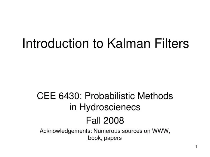
Introduction to Kalman Filters CEE 6430: Probabilistic Methods in Hydroscienecs Fall 2008 Acknowledgements: Numerous sources on WWW, book, papers
Overview • What could Kalman Filters be used for in Hydrosciences? • What is a Kalman Filter? • Conceptual Overview • The Theory of Kalman Filter (only the equations you need to use) • Simple Example (with lots of blah blah talk through handouts)
A “Hydro” Example • Suppose you have a hydrologic model that predicts river water level every hour (using the usual inputs). • You know that your model is not perfect and you don’t trust it 100%. So you want to send someone to check the river level in person. • However, the river level can only be checked once a day around noon and not every hour. • Furthermore, the person who measures the river level can not be trusted 100% either. • So how do you combine both outputs of river level (from model and from measurement) so that you get a ‘fused’ and better estimate? – Kalman filtering
What is a Filter by the way? Class – define mathematically what a filter is (make an analogy to a real filter) • Other applications of Kalman Filtering (or Filtering in general): • Your Car GPS (predict and update location) • Surface to Air Missile (hitting the target) • Ship or Rocket navigation (Appollo 11 used some sort of filtering to make sure it didn’t miss the Moon!)
The Problem in General (let’s get a little more technical) Black Box System Error Sources • System state cannot be measured directly • Need to estimate “optimally” from measurements Sometimes the system state and the measurement may be two different things (not like river level example) External Controls System System State (desired but not known) Optimal Estimate of System State Observed Measurements Measuring Devices Estimator Measurement Error Sources
What is a Kalman Filter? • Recursive data processing algorithm • Generates optimal estimate of desired quantities given the set of measurements • Optimal? • For linear system and white Gaussian errors, Kalman filter is “best” estimate based on all previous measurements • For non-linear system optimality is ‘qualified’ • Recursive? • Doesn’t need to store all previous measurements and reprocess all data each time step
Conceptual Overview • Simple example to motivate the workings of the Kalman Filter • The essential equations you need to know (Kalman Filtering for Dummies!) • Examples: Prediction and Correction
Conceptual Overview • Lost on the 1-dimensional line (imagine that you are guessing your position by looking at the stars using sextant) • Position – y(t) • Assume Gaussian distributed measurements y
Conceptual Overview State space – position Measurement - position Sextant is not perfect • Sextant Measurement at t1: Mean = z1 and Variance = z1 • Optimal estimate of position is: ŷ(t1) = z1 • Variance of error in estimate: 2x(t1) = 2z1 • Boat in same position at time t2 - Predicted position is z1
Conceptual Overview prediction ŷ-(t2) State (by looking at the stars at t2) Measurement usign GPS z(t2) • So we have the prediction ŷ-(t2) • GPS Measurement at t2: Mean = z2 and Variance = z2 • Need to correct the prediction by Sextant due to measurement to get ŷ(t2) • Closer to more trusted measurement – should we do linear interpolation?
Conceptual Overview prediction ŷ-(t2) Kalman filter helps you fuse measurement and prediction on the basis of how much you trust each (I would trust the GPS more than the sextant) corrected optimal estimate ŷ(t2) measurement z(t2) • Corrected mean is the new optimal estimate of position (basically you’ve ‘updated’ the predicted position by Sextant using GPS • New variance is smaller than either of the previous two variances
Conceptual Overview(The Kalman Equations) • Lessons so far: Make prediction based on previous data - ŷ-, - Take measurement – zk, z Optimal estimate (ŷ) = Prediction + (Kalman Gain) * (Measurement - Prediction) Variance of estimate = Variance of prediction * (1 – Kalman Gain)
Conceptual Overview What if the boat was now moving? ŷ(t2) Naïve Prediction (sextant) ŷ-(t3) • At time t3, boat moves with velocity dy/dt=u • Naïve approach: Shift probability to the right to predict • This would work if we knew the velocity exactly (perfect model)
Conceptual Overview Naïve Prediction ŷ-(t3) But you may not be so sure about the exact velocity ŷ(t2) Prediction ŷ-(t3) • Better to assume imperfect model by adding Gaussian noise • dy/dt = u + w • Distribution for prediction moves and spreads out
Conceptual Overview Corrected optimal estimate ŷ(t3) Updated Sextant position using GPS Measurement z(t3) GPS Prediction ŷ-(t3) Sextant • Now we take a measurement at t3 • Need to once again correct the prediction • Same as before
Conceptual Overview • Lessons learnt from conceptual overview: • Initial conditions (ŷk-1 and k-1) • Prediction (ŷ-k , -k) • Use initial conditions and model (eg. constant velocity) to make prediction • Measurement (zk) • Take measurement • Correction (ŷk , k) • Use measurement to correct prediction by ‘blending’ prediction and residual – always a case of merging only two Gaussians • Optimal estimate with smaller variance
Blending Factor • If we are sure about measurements: • Measurement error covariance (R) decreases to zero • K decreases and weights residual more heavily than prediction • If we are sure about prediction • Prediction error covariance P-k decreases to zero • K increases and weights prediction more heavily than residual
Correction (Measurement Update) Prediction (Time Update) (1) Compute the Kalman Gain (1) Project the state ahead K = P-kHT(HP-kHT + R)-1 ŷ-k = Ayk-1 + Buk (2) Update estimate with measurement zk (2) Project the error covariance ahead ŷk = ŷ-k + K(zk - H ŷ-k ) P-k = APk-1AT + Q (3) Update Error Covariance Pk = (I - KH)P-k The set of Kalman Filtering Equations in Detail
Assumptions behind Kalman Filter • The model you use to predict the ‘state’ needs to be a LINEAR function of the measurement (so how do we use non-linear rainfall-runoff models?) • The model error and the measurement error (noise) must be Gaussian with zero mean
What if the noise is NOT Gaussian? Given only the mean and standard deviation of noise, the Kalman filter is the best linear estimator. Non-linear estimators may be better. Why is Kalman Filtering so popular? · Good results in practice due to optimality and structure. · Convenient form for online real time processing. · Easy to formulate and implement given a basic understanding. · Measurement equations need not be inverted. ALSO popular in hydrosciences, weather/oceanography/ hydrologic modeling, data assimilation
Now ..to understand the jargons (You may begin the handouts) • First read the hand out by PD Joseph • Next, read the hand out by Welch and Bishop titled ‘An Introduction to the Kalman Filter’. (you can skip pages 4-5, 7-11). Pages 7-11 are on ‘Extended Kalman Filtering’ (for non-linear systems). Read the solved example from pages 11-16.
Homework (conceptual) • Explain in NO MORE THAN 1 PAGE the example that you read from pages 11-16 in the handout by Welch and Bishop. Basically, I want you to give me a simple conceptual overview of why and how ‘filtering’ was applied using the previous analogy on a boat lost in sea. • DUE – Same date as the Class project report. • EXTRA CREDIT 5% marks– If you review (3-4 pages) the classic paper in 1960 by Kalman (hand out) • EXTRA CREDIT 5% marks – if you turn in a detailed summary of the STEVE software (pros/cons, what it is etc.)
References • Kalman, R. E. 1960. “A New Approach to Linear Filtering and Prediction Problems”, Transaction of the ASME--Journal of Basic Engineering, pp. 35-45 (March 1960). • Welch, G and Bishop, G. 2001. “An introduction to the Kalman Filter”, http://www.cs.unc.edu/~welch/kalman/ By the way Dr. Rudolf Kalman is alive and living well today