Chapter 12
550 likes | 945 Views
Example: Ride Em Cowboy! M/D/1 Queuing System. The mechanical pony ride machine at the ... wanting to ride the pony arrive according to a Poisson distribution ...

Chapter 12
E N D
Presentation Transcript
- Slides Prepared by
JOHN S. LOUCKS
St. Edward�s University
Slide 2:Chapter 12 Waiting Line Models
The Structure of a Waiting Line System Queuing Systems Queuing System Input Characteristics Queuing System Operating Characteristics Analytical Formulas Single-Channel Waiting Line Model with Poisson Arrivals and Exponential Service Times Multiple-Channel Waiting Line Model with Poisson Arrivals and Exponential Service Times Economic Analysis of Waiting Lines
Slide 3:Structure of a Waiting Line System
Queuing theory is the study of waiting lines. Four characteristics of a queuing system are: the manner in which customers arrive the time required for service the priority determining the order of service the number and configuration of servers in the system.
Slide 4:Structure of a Waiting Line System
Distribution of Arrivals Generally, the arrival of customers into the system is a random event. Frequently the arrival pattern is modeled as a Poisson process. Distribution of Service Times Service time is also usually a random variable. A distribution commonly used to describe service time is the exponential distribution.
Slide 5:Structure of a Waiting Line System
Queue Discipline Most common queue discipline is first come, first served (FCFS). An elevator is an example of last come, first served (LCFS) queue discipline. Other disciplines assign priorities to the waiting units and then serve the unit with the highest priority first.
Slide 6:Structure of a Waiting Line System
Single Service Channel Multiple Service Channels S1 S1 S2 S3 Customer leaves Customer leaves Customer arrives Customer arrives Waiting line Waiting line System System
Slide 7:Queuing Systems
A three part code of the form A/B/k is used to describe various queuing systems. A identifies the arrival distribution, B the service (departure) distribution and k the number of channels for the system. Symbols used for the arrival and service processes are: M - Markov distributions (Poisson/exponential), D - Deterministic (constant) and G - General distribution (with a known mean and variance). For example, M/M/k refers to a system in which arrivals occur according to a Poisson distribution, service times follow an exponential distribution and there are k servers working at identical service rates.
Slide 8:Queuing System Input Characteristics
??????? = the average arrival rate 1/? = the average time between arrivals � = the average service rate for each server 1/� = the average service time ?? = the standard deviation of the service time
Slide 9:Queuing System Operating Characteristics
P0 = probability the service facility is idle Pn = probability of n units in the system Pw = probability an arriving unit must wait for service Lq = average number of units in the queue awaiting service L = average number of units in the system Wq = average time a unit spends in the queue awaiting service W = average time a unit spends in the system
Slide 10:Analytical Formulas
For nearly all queuing systems, there is a relationship between the average time a unit spends in the system or queue and the average number of units in the system or queue. These relationships, known as Little's flow equations are: L = ?W and Lq = ?Wq
Slide 11:Analytical Formulas
When the queue discipline is FCFS, analytical formulas have been derived for several different queuing models including the following: M/M/1 M/M/k M/G/1 M/G/k with blocked customers cleared M/M/1 with a finite calling population Analytical formulas are not available for all possible queuing systems. In this event, insights may be gained through a simulation of the system.
Slide 12:M/M/1 Queuing System
Single channel Poisson arrival-rate distribution Exponential service-time distribution Unlimited maximum queue length Infinite calling population Examples: Single-window theatre ticket sales booth Single-scanner airport security station
Slide 13:Example: SJJT, Inc. (A)
M/M/1 Queuing System Joe Ferris is a stock trader on the floor of the New York Stock Exchange for the firm of Smith, Jones, Johnson, and Thomas, Inc. Stock transactions arrive at a mean rate of 20 per hour. Each order received by Joe requires an average of two minutes to process. Orders arrive at a mean rate of 20 per hour or one order every 3 minutes. Therefore, in a 15 minute interval the average number of orders arriving will be ? = 15/3 = 5.
Slide 14:Example: SJJT, Inc. (A)
Arrival Rate Distribution Question What is the probability that no orders are received within a 15-minute period? Answer P (x = 0) = (50e -5)/0! = e -5 = .0067
Slide 15:Example: SJJT, Inc. (A)
Arrival Rate Distribution Question What is the probability that exactly 3 orders are received within a 15-minute period? Answer P (x = 3) = (53e -5)/3! = 125(.0067)/6 = .1396
Slide 16:Example: SJJT, Inc. (A)
Arrival Rate Distribution Question What is the probability that more than 6 orders arrive within a 15-minute period? Answer P (x > 6) = 1 - P (x = 0) - P (x = 1) - P (x = 2) - P (x = 3) - P (x = 4) - P (x = 5) - P (x = 6) = 1 - .762 = .238
Slide 17:Example: SJJT, Inc. (A)
Service Rate Distribution Question What is the mean service rate per hour? Answer Since Joe Ferris can process an order in an average time of 2 minutes (= 2/60 hr.), then the mean service rate, �, is � = 1/(mean service time), or 60/2. m = 30/hr.
Slide 18:Example: SJJT, Inc. (A)
Service Time Distribution Question What percentage of the orders will take less than one minute to process? Answer Since the units are expressed in hours, P (T < 1 minute) = P (T < 1/60 hour). Using the exponential distribution, P (T < t ) = 1 - e-�t. Hence, P (T < 1/60) = 1 - e-30(1/60) = 1 - .6065 = .3935 = 39.35%
Slide 19:Example: SJJT, Inc. (A)
Service Time Distribution Question What percentage of the orders will be processed in exactly 3 minutes? Answer Since the exponential distribution is a continuous distribution, the probability a service time exactly equals any specific value is 0 .
Slide 20:Example: SJJT, Inc. (A)
Service Time Distribution Question What percentage of the orders will require more than 3 minutes to process? Answer The percentage of orders requiring more than 3 minutes to process is: P (T > 3/60) = e-30(3/60) = e -1.5 = .2231 = 22.31%
Slide 21:Example: SJJT, Inc. (A)
Average Time in the System Question What is the average time an order must wait from the time Joe receives the order until it is finished being processed (i.e. its turnaround time)? Answer This is an M/M/1 queue with ? = 20 per hour and ? = 30 per hour. The average time an order waits in the system is: W = 1/(� - ? ) = 1/(30 - 20) = 1/10 hour or 6 minutes
Slide 22:Example: SJJT, Inc. (A)
Average Length of Queue Question What is the average number of orders Joe has waiting to be processed? Answer Average number of orders waiting in the queue is: Lq = ?2/[�(� - ?)] = (20)2/[(30)(30-20)] = 400/300 = 4/3
Slide 23:Example: SJJT, Inc. (A)
Utilization Factor Question What percentage of the time is Joe processing orders? Answer The percentage of time Joe is processing orders is equivalent to the utilization factor, ?/?. Thus, the percentage of time he is processing orders is: ?/? = 20/30 = 2/3 or 66.67%
Slide 24:Example: SJJT, Inc. (A)
Formula Spreadsheet
Slide 25:Example: SJJT, Inc. (A)
Spreadsheet Solution
Slide 26:M/M/k Queuing System
Multiple channels (with one central waiting line) Poisson arrival-rate distribution Exponential service-time distribution Unlimited maximum queue length Infinite calling population Examples: Four-teller transaction counter in bank Two-clerk returns counter in retail store
Slide 27:Example: SJJT, Inc. (B)
M/M/2 Queuing System Smith, Jones, Johnson, and Thomas, Inc. has begun a major advertising campaign which it believes will increase its business 50%. To handle the increased volume, the company has hired an additional floor trader, Fred Hanson, who works at the same speed as Joe Ferris. Note that the new arrival rate of orders, ? , is 50% higher than that of problem (A). Thus, ? = 1.5(20) = 30 per hour.
Slide 28:Example: SJJT, Inc. (B)
Sufficient Service Rate Question Why will Joe Ferris alone not be able to handle the increase in orders? Answer Since Joe Ferris processes orders at a mean rate of � = 30 per hour, then ? = � = 30 and the utilization factor is 1. This implies the queue of orders will grow infinitely large. Hence, Joe alone cannot handle this increase in demand.
Slide 29:Example: SJJT, Inc. (B)
Probability of n Units in System Question What is the probability that neither Joe nor Fred will be working on an order at any point in time?
Slide 30:Example: SJJT, Inc. (B)
Probability of n Units in System (continued) Answer Given that ? = 30, � = 30, k = 2 and (? /�) = 1, the probability that neither Joe nor Fred will be working is: = 1/[(1 + (1/1!)(30/30)1] + [(1/2!)(1)2][2(30)/(2(30)-30)] = 1/(1 + 1 + 1) = 1/3 = .333
Slide 31:Example: SJJT, Inc. (B)
Average Time in System Question What is the average turnaround time for an order with both Joe and Fred working?
Slide 32:Example: SJJT, Inc. (B)
Average Time in System (continued) Answer The average turnaround time is the average waiting time in the system, W. ?�(? /�)k (30)(30)(30/30)2 Lq = P0 = (1/3) = 1/3 (k-1)!(k� - ? )2 (1!)((2)(30)-30))2 L = Lq + (? /�) = 1/3 + (30/30) = 4/3 W = L/?????(4/3)/30 = 4/90 hr. = 2.67 min.
Slide 33:Example: SJJT, Inc. (B)
Average Length of Queue Question What is the average number of orders waiting to be filled with both Joe and Fred working? Answer The average number of orders waiting to be filled is Lq. This was calculated earlier as 1/3 .
Slide 34:Example: SJJT, Inc. (B)
Formula Spreadsheet
Slide 35:Example: SJJT, Inc. (B)
Spreadsheet Solution
Slide 36:Example: SJJT, Inc. (B)
Creating Special Excel Function to Compute P0 Select the Tools pull-down menu Select the Macro option Choose the Visual Basic Editor When the Visual Basic Editor appears Select the Insert pull-down menu Choose the Module option When the Module sheet appears Enter Function Po (k,lamda,mu) Enter Visual Basic program (on next slide) Select the File pull-down menu Choose the Close and Return to MS Excel option
Slide 37:Example: SJJT, Inc. (B)
Visual Basic Module for P0 Function Function Po(k, lamda, mu) Sum = 0 For n = 0 to k - 1 Sum = Sum + (lamda/mu) ^ n / Application.Fact(n) Next Po = 1/(Sum+(lamda/mu)^k/Application.Fact(k))* (k*mu/(k*mu-lamda))) End Function
Slide 38:Example: SJJT, Inc. (C)
Economic Analysis of Queuing Systems The advertising campaign of Smith, Jones, Johnson and Thomas, Inc. (see problems (A) and (B)) was so successful that business actually doubled. The mean rate of stock orders arriving at the exchange is now 40 per hour and the company must decide how many floor traders to employ. Each floor trader hired can process an order in an average time of 2 minutes.
Slide 39:Example: SJJT, Inc. (C)
Economic Analysis of Queuing Systems Based on a number of factors the brokerage firm has determined the average waiting cost per minute for an order to be $.50. Floor traders hired will earn $20 per hour in wages and benefits. Using this information compare the total hourly cost of hiring 2 traders with that of hiring 3 traders.
Slide 40:Example: SJJT, Inc. (C)
Economic Analysis of Waiting Lines Total Hourly Cost = (Total salary cost per hour) + (Total hourly cost for orders in the system) = ($20 per trader per hour) x (Number of traders) + ($30 waiting cost per hour) x (Average number of orders in the system) = 20k + 30L. Thus, L must be determined for k = 2 traders and for k = 3 traders with ? = 40/hr. and ? = 30/hr. (since the average service time is 2 minutes (1/30 hr.).
Slide 41:Example: SJJT, Inc. (C)
Cost of Two Servers P0 = 1 / [1+(1/1!)(40/30)]+[(1/2!)(40/30)2(60/(60-40))] = 1 / [1 + (4/3) + (8/3)] = 1/5
Slide 42:Example: SJJT, Inc. (C)
Cost of Two Servers (continued) Thus, ?�(? /�)k (40)(30)(40/30)2 Lq = P0 = (1/5) = 16/15 (k-1)!(k� -? )2 1!(60-40)2 L = Lq + (? /�) = 16/15 + 4/3 = 12/5 Total Cost = (20)(2) + 30(12/5) = $112.00 per hour
Slide 43:Example: SJJT, Inc. (C)
Cost of Three Servers P0 = 1/[[1+(1/1!)(40/30)+(1/2!)(40/30)2]+ [(1/3!)(40/30)3(90/(90-40))] ] = 1 / [1 + 4/3 + 8/9 + 32/45] = 15/59
Slide 44:Example: SJJT, Inc. (C)
Cost of Three Servers (continued) (30)(40)(40/30)3 Hence, Lq = (15/59) = 128/885 = .1446 (2!)(3(30)-40)2 Thus, L = 128/885 + 40/30 = 1308/885 (= 1.4780) Total Cost = (20)(3) + 30(1308/885) = $104.35 per hour
Slide 45:Example: SJJT, Inc. (C)
System Cost Comparison Wage Waiting Total Cost/Hr Cost/Hr Cost/Hr 2 Traders $40.00 $82.00 $112.00 3 Traders 60.00 44.35 104.35 Thus, the cost of having 3 traders is less than that of 2 traders.
Slide 46:M/D/1 Queuing System
Single channel Poisson arrival-rate distribution Constant service time Unlimited maximum queue length Infinite calling population Examples: Single-booth automatic car wash Coffee vending machine
Slide 47:Example: Ride �Em Cowboy!
M/D/1 Queuing System The mechanical pony ride machine at the entrance to a very popular J-Mart store provides 2 minutes of riding for $.50. Children (accompanied of course!) wanting to ride the pony arrive according to a Poisson distribution with a mean rate of 15 per hour. a) What fraction of the time is the pony idle? b) What is the average number of children waiting to ride the pony? c) What is the average time a child waits for a ride?
Slide 48:Example: Ride �Em Cowboy!
Fraction of Time Pony is Idle l = 15 per hour m = 60/2 = 30 per hour Utilization = l/m = 15/30 = .5 Idle fraction = 1 � Utilization = 1 - .5 = .5
Slide 49:Example: Ride �Em Cowboy!
Average Number of Children Waiting for a Ride Average Time a Child Waits for a Ride (or 1 minute)
Slide 50:M/G/k Queuing System
Multiple channels Poisson arrival-rate distribution Arbitrary service times No waiting line Infinite calling population Example: Telephone system with k lines. (When all k lines are being used, additional callers get a busy signal.)
Slide 51:Example: Allen-Booth
M/G/k Queuing System Allen-Booth (A-B) is an OTC market maker. A broker wishing to trade a particular stock for a client will call on a firm like Allen-Booth to execute the order. If the market maker's phone line is busy, a broker will immediately try calling another market maker to transact the order. A-B estimates that on the average, a broker will try to call to execute a stock transaction every two minutes. The time required to complete the transaction averages 75 seconds. A-B has four traders staffing its phones. Assume calls arrive according to a Poisson distribution.
Slide 52:Example: Allen-Booth
This problem can be modeled as an M/G/k system with block customers cleared with: 1/l = 2 minutes = 2/60 hour l = 60/2 = 30 per hour 1/� = 75 sec. = 75/60 min. = 75/3600 hr. � = 3600/75 = 48 per hour
Slide 53:Example: Allen-Booth
% of A-B�s Potential Customers Lost Due to Busy Line First, we must solve for P0 where k = 4 1 P0 = 1 + (30/48) + (30/48)2/2! + (30/48)3/3! + (30/48)4/4! P0 = .536 continued
Slide 54:Example: Allen-Booth
% of A-B�s Potential Customers Lost Due to Busy Line (l/�)4 (30/48)4 Now, P4 = P0 = (.536) = .003 4! 24 � Thus, with four traders 0.3% of the potential customers are lost.
Slide 55:End of Chapter 12