Download
1 / 33
350 likes | 900 Views
Additive pattern database heuristics. Ariel Felner Bar-Ilan University. felner@cs.biu.ac.il September 2003 Joint work with Richard E. Korf Journal version submitted to JAIR. Available at: http://www.cs.biu.ac.il/~felner. A* and its variants.

E N D
Additive pattern database heuristics Ariel Felner Bar-Ilan University. felner@cs.biu.ac.il September 2003 Joint work with Richard E. Korf Journal version submitted to JAIR. Available at: http://www.cs.biu.ac.il/~felner
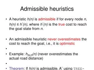
A* and its variants • A* is a best-firstsearch algorithm that uses f(n)=g(n)+h(n)as its cost function. Nodes are sorted in an open-list according to their f-value. • g(n)is the shortest known path between the initial node and the current node n. • h(n)is an admissible (lower bound) heuristic estimation from n to the goal node • A* is admissible, complete and optimally effective. [Pearl 84] • A* is memory limited. • IDA* is the linear-space version of A*.
How to improve search? • Enhanced algorithms: Perimeter-search, RBFS, Frontier-search etc, They all try to better explore the search tree. • Better heuristics:more parts of the search tree will be pruned. • In the 3rd Millennium we have very large memories. We can build large tables. • For enhanced algorithms: large open-lists or transposition tables. They store nodes explicitly. • A more intelligent way is to store general knowledge. We can do this with heuristics
Pattern databases • Many problems can be decomposed into subproblems that must be also solved. • The cost of a solution to a subproblem is a lower-bound on the cost of the complete solution. • Instead of calculating the solution on the fly, expand the whole state-space of the subproblem and store the solution to each state in a database. • These are called pattern databases
Non-additive pattern databases • Fringe database for the 15 puzzle by (Culberson and Schaeffer 1996). • Stores the number of moves including tiles not in the pattern • Rubik’s Cube. (Korf 1997) • The best way to combine different non-additive pattern databases is to take their maximum!! • These databases don’t scale up to large problems.
Additive pattern databases • We want to add values from different pattern databases. • There are two ways to build additive databases: • -> Statically-partitioned additive databases • -> Dynamically-partitioned additive databases. • We will present additive pattern databases for: • Tile puzzles • 4-peg towers of Hanoi problem • Multiple sequence-alignment problem • Vertex-cover • We will then present a general theory that discusses the conditions for additive pattern databases.
Statically-partitioned additive databases • These were created for the 15 and 24 puzzles (Korf & Felner 2002) • We statically partition the tiles into disjoint patterns and compute the cost of moving only these tiles into their goal states. • For the 15 puzzle: • 36,710 nodes. • 0.027 seconds. • 575 MB • For the 24 puzzle: • 360,892,479,671 • 2 days • 242 MB
Dynamically-partitioned additive databases • Statically-partition databases do not capture conflicts of tiles from different patterns. • We want to store as many pattern databases as possible and partition them to disjoint subproblems on the fly such the chosen partition will yield the best heuristic. • Suppose we take all possible pairs and build a graph such that tiles are nodes and edges are the pairwise cost of the two nodes (tiles) incident with that edge. 2 1 2 1 1 2 1 3 4 1
Mutual cost graph • Maximum matching to the above pairwise-graph will yield the best dynamic partitioning. • With larger groups (triples, quadruples) this graph can be called the mutual-cost graph. • Maximum-matching on the mutual-cost graph is an admissible heuristic. • In practice we can use only the addition above the Manhattan-distance. In that case many edges disappear. This graph is called the conflict-graph
Weighted vertex-cover (WVC) • For the special case of the tile puzzle we can do better. • An edge {x, y}=2 means (x+y>=2) • For each edge, one tile should move at least two more moves than its MD, yielding a constraint: (x>=2 or y>=2) • Divide the costs by two then this is actually a vertex-cover of the conflict graph. • Will produce a heuristic of 4 for the shown graph. • With hyperedges and larger costs we get weighted vertex-cover. 2 2 2 3 2 1
Weighted vertex-cover (cont.) • A hyperedge of three tiles (x,y,z) with a cost of 4 means that (x+y+z>=4) but also that: • (x>=4) or (y>=4) or (z>=4) or (x>=2 and y>=2) or (x>=2 and z>=2) or (y>=2 and z>=2) • WVC is NP-complete. Why? Because simple VC is NPC and is a special case of WVC. • Our graph for the tile puzzles is very sparse. We only had few edges with costs above MD!!
Summary: DDB for the tile puzzle • Before the search: • Store all pairwise, triple, quadruple conflict in a pattern database. • During the search: for each node of the search tree: • 1) build the conflict-graph • 2) Calculate WVC of the conflict-graph as an admissible heuristic. • Many domain dependent enhancements are applicable. e.g. only incremental changes etc,
Experimental Results:15 puzzle Fives Sixes Seven+Eight
Results: 24 puzzle. • For the 24 puzzle we compared the SDB of sixes with the DDB of pairs + triples on 10 random instances. • The relative advantage of the SDB decreases when the problem scales up • What will happen for the 6x6 35 puzzle???
35 puzzle We sampled 10 Billion random states and calculated their heuristic. The table was created by the method presented by Korf, Reid and Edelkamp. (AIJ 129, 2001)
Tile puzzles: Summary • The relative advantage of the SDB over DDB decreases over time. • For the 15 puzzle 1/2 of the domain is stored. • For the 24 puzzle 1/4 of the domain is stored. • For the 35 puzzle 1/7 of the domain is stored. • The memory needed by the DDB was 100 times smaller than that of the SDB!!
4-peg Towers of Hanoi (TOH) • There is a conjecture about the length of optimal path but it was not proven. • Systematic search is the only way to solve this problem or to verify the conjecture. • There are too many cycles. IDA* as a DFS will not prune these cycle. Therefore, A* (actually frontier A* [Korf 2000]) was used.
Heuristics for the TOH • Infinite peg heuristic (INP): Each disk moves to its own temporary peg. • Additive pattern databases: • Partition the disks into disjoint sets. 8 and 7 for example in the 15-disk problem. • Store the cost of the complete state space of each set in a pattern database table. • The n-disk problem contains 4^n states and 2n bits suffice to store each state.
Pattern databases for TOH • There is only one database for a pattern of size n. • A pattern database of size n also contains a pattern database of size m<n by simply assigning the n-m larger disks to the goal peg. • The largest databases that we stored was of size 14 • 4^14=256MB if each state needs a byte. • To solve the 15 disks problem we can split the disks into 14-1, 13-2 or 12-3 disks. • The SDB will use the same partition at all times. • The DDB looks on all possible partitions and chooses the partition with the best heuristic. • There are (14*13*12)/6=364 different 12-3 splits.
Vertex-Cover (VC) 0 1 • Given a graph we want the minimal set of vertices such that they cover all the edges. • VC was one of the first problems that was proved to be NP-complete. • Search tree: • At each level, either include or exclude a vertex. • Improvements: • If a node is excluded, all its neighbors bust be included. • Dealing with degree-0 and degree-1 vertices. 2 3 R X:0 V:1,2,3 V:0 V:0,2 X:1 V:0,1
Heuristics for VC • The included edges form the g part of: f=g+h. • We want an admissible heuristic of the free vertices. • Pairwise heuristic: A maximum-matching of the free-graph. • For a triangle we can add two to the heuristic. • In general, a clique of size k contributes k-1 to h. • So: partition the free-graph into disjoint cliques and sum up their heuristics. VC EX 1 3 2 4 Free vertices
Additive pattern databases • Cliqueis NP-complete. However, in random graphs, cliques of size 5 and larger are rare. Thus, it is easy to finds small cliques • Pattern databases: Instead of finding the cliques on the fly we identify them before the search and store them in a pattern database. We stored cliques of size 4 or smaller. • During the search we need to retrieve disjoint cliques from the pattern database.
VC:additive heuristics • 1) We match the free graph against the database and form a hyper-graph (conflict-graph) such that each hyper-edges corresponds to a clique in the free-graph. • 2) A maximum-matching (MM) of this graph is an admissible heuristic of the free graph. • Since maximum-matching is NP-complete, we can settle for maximal-matching. • Dynamic partitioning: do the above process for each new node of the search tree.
VC: heuristics (cont.) • Static partitioning: Do the above process only once and use these cliques for al the nodes of the search tree. • A clique of size k contributes k-m-1 to the heuristic given that m vertices were already included in the partial vertex-cover. • Once again, the static partitioning is faster but is less accurate since we are forced to use the same partitioning.
VC: results • The results are on random graphs of size 150 and an average degree of 16. • When we added our dynamic database to the best proven tree search algorithm we further improved the running time by a fact or more than 10.
Conclusions and Summary • In general: Additivity can be applied whenever a problem can be decomposed into disjoint subproblems such that the sum of the costs is a lower bound on cost of the complete problem. • Additive databases is a special case of additive heuristic where we save the heuristics in a table.
Theory: definitions • A problem consists a set of objects. • A pattern is a subset of objects of the problem • Asubproblem is associated with a pattern. • The cost of solving the subproblem is a lower bound on the cost of the complete problem. • Patterns are disjoint if they have no objects in common • The costs of subproblems are additive if their sum is a lower bound on the cost of solving them together
Condition for additivity • Additivity can be applied if the cost of a subproblem is composed from costs of objects from corresponding pattern only • Permutation puzzles • The domain includes permutations of objects and operators that map one permutation to another. • For the tile puzzles and TOH, every operator moves only one tile and the above claim is valid. • Rubik’s cube and a disjoint version of pattern databases of Culberson and Schaeffer (96) are counter examples.
Algorithm schema: static database • In the precomputation phase do: • Partition the objects into disjoint patterns • Solve the corresponding subproblems and store the costs in a database. • In the search phase do: • For each node retrieve the values of the costs of the subproblems and sum them up for anadmissible heuristic
Algorithm schema: dynamic database • In the precomputation phase do: • For each pattern to be used, solve the corresponding subproblem and store the costs in a database. • In the search phase do: • For each node retrieve the values of the costs of the all subproblems from the database. • Find a set of disjoint subproblems such that the sum of the costs is maximized. • There are of course many domain dependent enhancements.
Discussion • The dynamic partitioned database is more accurate at a cost of larger constant time per node. • Adding more patterns to a system is beneficial up to a certain point. • That point can be currently found by a trial and error process. • Memory is also an issue. Different techniques have different memory requirements.
Summary • Static databases were better for the tile puzzles and multiple sequence alignment. • Dynamic databases were better for the vertex-cover problem and for the towers of Hanoi. • Future work: • Automatically find the best static partition. • Better ways of finding the best dynamic partition. • Other problems. • Given a certain amount of memory how to make the best use of it.