Download
1 / 24
240 likes | 311 Views
Deciding separation formulas with SAT. Ofer Strichman Sanjit A. Seshia Randal E. Bryant School of Computer Science, Carnegie Mellon University. Separation predicates. Predicates of the form x 1 < x 2 + c and x 1 x 2 + c where c is a constant

E N D
Deciding separation formulas with SAT Ofer Strichman Sanjit A. Seshia Randal E. Bryant School of Computer Science, Carnegie Mellon University
Separation predicates • Predicates of the form x1< x2+ c and x1x2+ c where c is a constant • Also known as ‘difference predicates’ • We will consider x1,x2 as either real or integer variables • Used when proving formulas derived from Timed automata, Scheduling problems, and more • Pratt: “Most inequalities arising in verification are separation predicates”
Case splitting x2 x2 x1 x1 1 1 1 1 1 -3 x3 x3 Deciding separation via case-splitting (1/2) : x1 < x2 + 1 x2 < x3 + 1 (x3 < x1 -3 x3 < x1 +1) x1 < x2 + 1 x2 < x3 + 1 x3 < x1 +1 x1 < x2 + 1 x2 < x3 + 1 x3 < x1 -3 Theorem [Bellman, 57]: The formula is satisfiable iff the inequality graph does not contain a negative cycle.
1 5 -4 1 -3 Deciding separation via case-splitting (2/2) Bellman-Ford: Finding whether there is a negative cycle in a graph is polynomial • Overall complexity: O(2| |), due to case-splitting • Case-splitting is normally the bottleneck of decision procedures • Q: Is there an alternative to case-splitting ?
x1 – x3 < 0 x2 -x3 0 x2-x1 <0 1 0 Difference Decision Diagrams(DDD)(Møller, Lichtenberg, Andersen, Hulgaard, 1999) • Similar to BDDs, but the nodes are separation predicates • Ordering on variables determines order on predicates • Semi-canonical (i.e canonical when is a tautology or a contradiction) : !(x1 – x3 < 0) x2 -x3 0 !(x2-x1 <0) • Each path leading to ‘1’ is checked for consistency with ‘Bellman-Ford’ • Worst case – an exponential no. of such paths
’: x1 x2 1 1 2. Build the joint graph G: 1 -3 x3 Boolean encoding (take 1) : x1 < x2 + 1 x2 < x3 + 1 (x3 < x1 -3 x3 < x1 +1) 1. Encode: 3. Forbid ‘true’ assignment to negative simple cycles in G:
What about negations in ? The unsatisfiable formula : ¬(x1 < x2 x2 x1+1) is reduced to the satisfiable formula: 0 x1 x2 1 Legend: ‘<’ ‘’ Problem: our graph does not consider the polarity of the constraints.
x2 x1 -1 x1 x2 1 -1 1 3 -3 x3 x3 -1 x2 x1 1 -1 -3 1 3 x3 Solution #1: Consider both polarities x2 x1-1 Dual edges: x1 < x2+1 The joint graph:
Solution #2: Eliminate negations 1. Transform to Negation Normal Form (NNF), and eliminate negations by reversing inequality signs 2. Rewrite ‘>’ and ‘’ predicates as ‘<’ and ‘’, e.g. rewrite x1 > x2 + c as x2 < x1 – c Solution #2 results in a smaller number of constraints
Case splitting x1 x1 -3 -3 1 x3 x2 x3 x2 -1 x1 The joint graph G: -3 1 x3 x2 -1 G creates redundant constraints Problem: redundant constraints : (x1 < x2 -3 (x2<x3 –1 x3 < x1 +1))
Solution: Conjunctions Matrices (1/3) • Let dbe the DNF representation of • We only need to consider cycles that are in one of the clauses of d • Deriving dis exponential. But – • Knowing whether a given set of literals share a clause in dis polynomial, using Conjunctions Matrices
:l0 (l1(l2 l3)) l0 l1 l2 l3 1 1 1 l0 l1 l2 l3 M: l0 1 0 0 l1 1 0 1 l2 l3 1 0 1 Conjunctions Matrix Conjunctions Matrices (2/3) • Let be a formula in NNF. • Let liand ljbe two literals in . • The joining operandof liand ljis the lowest joint parent of liand ljin the parse tree of .
x0 x1 : x0 < x1 (x1<x2 (x2 < x3 x3 < x0)) x3 x2 Conjunctions Matrices (3/3) • Claim: A set of literals L={l0,l1…ln} share a clause in diff for allli,lj L, ij, M[li,lj] =1. • In our case the literals are separation predicates. • The entries in the conjunctions matrix correspond to ‘edges between edges’ • We can now consider only simple cycles that their correspondingMgraph form a clique.
Boolean encoding (take 2) 0. Normalize (eliminate negations) 1. Encode (replace each separation predicate with a Boolean var) 2. Build the joint inequality graph G 3. Add a constraint forbidding ‘true’ assignment to negative simple cycles in G that their corresponding Mform a clique.
..... ..... Compact representation of constraints (1/2) n diamonds 2nsimple cycles. Can we do better than that ? In many cases - yes. How? with variable elimination c2 c1 c1+ c2 c3 c4
c1 x1 x3 c2 c3 x2 x4 c1 + c3 x4 x1 c2 + c3 x4 x2 Compact representation of constraints (2/2) Quantifying out x3: • Worst case exponential no. of constraints • Complexity heavily depends on elimination order • Given a conjunctions matrix M, we add a constraint only if the joining operand of the two constraints is ‘’
Boolean encoding (take 3) 0. Normalize (eliminate negations) 1. Encode (replace each separation predicate with a Boolean var) 2. Build the joint inequality graph G 3. Eliminate all variables successively: • e1 and e2 are ingoing and outgoing edges of the eliminated variable, and • M[e1,e2]=1, and • the resulting edge ise3 then add to’ the constraint e1 e2e3 If
Extension to integer variables Given with integer separation predicates, derive R: • Declare all variables as real • Replace x1<x2 + c and x1x2 + c wherec is not an integer, with x1x2 + c • Replace each predicate x1<x2 + c with x1 x2 + c – 1 Theorem: is satisfiable iffR is satisfiable
Experimental results (1/3) d=2 ..... • n diamonds • Each diamond has 2d edges • Top and bottom paths in each diamond are disjointed. There are 2nconjoined cycles. • By adjusting the weights, we ensured that there is a single satisfying assignment.
Experimental results (2/3) ‘Diamond’ shape formulas • Results in seconds • Using variable elimination (rather than explicit cycle enumeration)
Experimental results (3/3) Symbolic simulation of hardware designs • Results in seconds • Using variable elimination (rather than explicit cycle enumeration)
Discussion and conclusions (1/2) • Procedures based on case-splitting can not scale • SAT methods can also be seen as ‘case-splitting’, but they split the domain, not the formula. As a result: • Pruning is easy • Learning is easy • Guidance is easy (“which case should we start with ?”)
Discussion and conclusions (2/2) • Both the reduction to SAT and solving the SAT instance are exponential • The reduction to SAT is the bottleneck of our procedure, whereas the resulting SAT instances are empirically easy to solve • The total time was shorter in all examples comparing to ICS and DDD’s • The decision procedure has recently been integrated into the theorem prover C-prover and the verification system Uclid