Download
1 / 47
470 likes | 637 Views
Simple extractors for all min-entropies and a new pseudo-random generator. Ronen Shaltiel Chris Umans. PRG. seed. pseudo-random bits. few truly random bits. many “ pseudo-random ” bits. Pseudo-Random Generators.

E N D
Simple extractors for all min-entropies and a new pseudo-random generator Ronen Shaltiel Chris Umans
PRG seed pseudo-random bits few truly random bits many“pseudo-random” bits Pseudo-Random Generators Hardness vs. Randomness paradigm: [BM,Y,S] Construct PRGs assuming hard functions. fEXP hard (on worst case) for small circuits. [NW88,BFNW93,I95,IW97,STV99,ISW99,ISW00] Use a short “seed” of very few truly random bits to generate a long string of pseudo-random bits. Pseudo-Randomness: No small circuit can distinguish truly random bits from pseudo-random bits. Nisan-Wigderson setting: The generator is more powerful than the circuit. (i.e., PRG runs in time n5 for circuits of size n3).
A sample from a physical source of randomness. A high (min)-entropy distribution. statistically close to uniform distribution. Randomness Extractors [NZ] Extractors extract many random bits from arbitrary distributions which contain sufficient randomness. Ext imperfect randomness random bits Impossible for deterministic procedures!
imperfect randomness short seed Randomness Extractors [NZ] Extractors use a short seed of truly random bits extract many random bits from arbitrary distributions which contain sufficient randomness. Ext random bits Extractors have many applications! A lot of work on explicit constructions [vN53,B84, SV86,Z91,NZ93,SZ94,Z96,T96,T99,RRV99,ISW00, RSW00,TUZ01,TZS02]. Survey available from my homepage.
PRGs Extractors Pseudo-random bits random bits hard function imperfect randomness PRG Ext short seed short seed Trevisan’s argument Trevisan’s argument: Every PRG construction with certain relativization properties is also an extractor. Extractors using the Nisan-Wigderson generator: [Tre99,RRV99,ISW00,TUZ01].
The method of Ta-Shma, Zuckerman and Safra [TZS01] • Use Trevisan’s argument to give a new method for constructing extractors. • Extractors by solving a “generalized list-decoding” problem. (List-decoding already played a role in this area [Tre99,STV99]). • Solution inspired by list-decoding algorithms for Reed-Muller codes [AS,STV99]. • Simple and direct construction.
Our results • Use the ideas of [TZS01] in an improved way: • Simple and direct extractors for all min-entropies. (For every a>0, seed=(1+a)(log n), output=k/(log n)O(a) .) • New list-decoding algorithm for Reed-Muller codes [AS97,STV99]. • Trevisan’s argument “the other way”: • New PRG construction. (Does not use Nisan-Wigderson PRG). • Optimal conversion of hardness into pseudo-randomness. (HSG construction using only “necessary” assumptions). • Improved PRG's for nondeterministic circuits (Consequence: better derandomization of AM). • Subsequent paper [Uma02] gives quantitive improvements for PRGs.
PRG short seed pseudo-random bits n bits n10 bits Goal: Construct pseudo-random generators • We’re given a hard function f on n bits. • We want to construct a PRG.
x Truth table of f A naive idea f(x)..f(x+n10) G outputs n10 successive values of f G(x)=f(x),f(x+1),..,f(x+n10) Previous: Make positions as independent as possible. [TZS01]: Make positions as dependent as possible.
fisn’t hard Gisn’t pseudo-random f is hard G is pseudo-random Want to prove
f is hard G is pseudo-random fisn’t hard Use P to compute f Exists next-bit predictorP for G Gisn’t pseudo-random Outline of Proof
Next-Bit Predictors fisn’t hard Use P to compute f Exists next-bit predictorP for G Gisn’t pseudo-random • By the hybrid argument, there’s a small circuit P which predicts the next bit given the previous bits. • P(prefix)=next bit with probability ½+ε. f(x)..f(x+i-1) f(x+i)
Showing that f is easy fisn’t hard Use P to compute f Exists next-bit predictorP for G Gisn’t pseudo-random To show that f is easy we’ll use P to construct a small circuit for f. • Circuits can use “non-uniform advice”. • We can choose nO(1) inputs and query f on these inputs.
We need to design an algorithm that: Queries f at few positions. (poly(n)). Uses the next-bit predictor P. Computes f everywhere. (on all 2n positions). Rules of the game fisn’t hard Use P to compute f Exists next-bit predictorP for G Gisn’t pseudo-random
Computing f using few queries fisn’t hard Use P to compute f Exists next-bit predictorP for G Gisn’t pseudo-random Simplifying assumption: P(prefix)=next bit with probability 1. Queries (non-uniform advice) f(0),..,f(i-1) - n10 bits Use P to compute f(i),f(i+1),f(i+2)… Compute f everywhere f(0)…f(i-1) f(1)……f(i) f(2)..f(i+1) f(i) f(i+1) f(i+2)
We need to design an algorithm that: Queries f at few positions. (poly(n)). Uses the next-bit predictor P. Computes f everywhere. (on all 2n positions). Rules of the game fisn’t hard Use P to compute f Exists next-bit predictorP for G Gisn’t pseudo-random *To get a small circuit we also need that for every x, f(x) can be computed in time nO(1) given the non-uniform advice.
f(x)..f(x+i-1) Prefix f(x+i) A Problem: The predictor makes errors We’ve made a simplifying assumption that: Prx[P(prefix)=next bit] = 1 We are only guaranteed that: Prx[P(prefix)=next bit] > ½+ε Use Error-Correcting techniques to recover from errors! Error: cannot Continue! f(0)…f(i-1) f(1)……f(i)
Using multivariate polynomials A line: One Dimension 2n The function f
2n/2 2n/2 Using multivariate polynomials A cube: many dimensions w.l.o.g f(x1,..,xd) is a low degree polynomial in d variables* x1 f(x1,x2) x2 *Low degree extension [BF]: We take a field F with about 2n/delements and extend f to a degree about 2n/dpolynomial in d variables.
Problem: No natural meaning to successive in many dimensions. Successive in [TZS01]: move one point right. The Generator: G(x1,x2)=f(x1,x2)..f(x1,x2+n10) X1 X2 Adjusting to Many Dimensions 2n/2 f(x1,x2)..f(x1,x2+n10)
Apply the Predictor in parallel along a random line. With high probability we get (½+ε)-fraction of correct predictions.* Apply error correction: Learn all points on line v v x v v v v v v v x v v v v v x v v v v v v v v x v Decoding Errors 2n/2 A restriction of f to a line: A univariate polynomial! x v v x If #errors is small (<25%) then it is possible to recover the correct values. The predictor is only correct with probability ½+ε . May make almost 50% errors. v Low degree univariate polynomials have error-correcting properties! Basic idea: Use decoding algorithms for Reed-Solomon codes to decode and continue. x v v x *By pairwise independence properties of random lines.
Coding Theory: Not enough information on on the line to uniquely decode. It is possible to List-Decode to get few polynomials one of which is correct [S97]. [TZS01]: Use additional queries to pin down the correct polynomial. x v v x v x v v x Too many errors We also have the information we previously computed! 2n/2
Lines: deg. 1 polynomials: L(t)=at+b Curves: higher deg. (nO(1))C(t)=artr+ar-1tr-1..+a0 Curves Instead of Lines 2n/2 • Observation: f restricted to a low-degree curve is still a low-degree univariate polynomial. • Points on degree r curve are r-wise independent. (crucial for analysis).
Curve passes through: Few (random) points Successive points. A special curve with intersection properties. 2n/2 This curve intersects itself when moved!
No errors! Previously computed. (½+ε)-fraction of correct predictions. Recovering From Errors 2n/2 Just like before: Query n10 successive curves. Apply the predictor in parallel.
No errors! Previously computed. Lemma: += (½+ε)-fraction of correct predictions. Recovering From Errors 2n/2 Given: - “Noisy” predicted values. - Few correct values. We can correct!
Lemma: += Recovering From Errors 2n/2 We implemented an errorless Predictor! Warning: This presentation is oversimplified. The lemma works only for randomly placed points. Actual solution is slightly more complicated and uses two “interleaved” curves. Given: - “Noisy” predicted values. - Few correct values. We can correct!
Story so far… • We can “error-correct” a predictor that makes errors. • Coding Theory: Our strategy gives a new list-decoding algorithm for Reed-Muller codes [AS97,STV99]. Short version
List decoding Given a corrupted message p: Pr[p(x)=f(x)]>ε Output f1,..,ft s.t. f in list.
Our setup: List decoding with predictor Given a predictorP: Pr[P(f(x-1),f(x-2),..,f(x-i))=f(x)]>ε Use k queries to compute f everywhere.
Our setup: List decoding with predictor Given a predictorP: Pr[P(x,f(x-1),f(x-2),..,f(x-i))=f(x)]>ε Use k queries to compute f everywhere. The decoding scenario is a special case when i=0 (predictor from empty prefix).
Our setup: List decoding with predictor Given a predictorP: Pr[P(x,f(x-1),f(x-2),..,f(x-i))=f(x)]>ε Use k queries to compute f everywhere. To list-decode output all possible f’s for all 2k possible answers to queries.
Want: nO(1) Make: n10 · |Curve| n10 How many queries? 2n/2 2n/2 Want to use short curves.
1 dimension: 2n 2 dimensions: 2n/2 3 dimensions: 2n/3 Using many dimensions d dimensions: 2n/d d=Ω(n/log(n))=> length = nO(1)
Conflict? Many Dimensions One Dimension Error correction. Few queries. Natural meaning to successive. We’d like to have both!
Fd Vector-Space. Base Field F. Fd Extension Field of F. Multiplicative group has a generator g. Fd \ 0={1,g,g2,g3,…} Successor(v)=g·v Covers the space. A different Successor Function 1 g g2 g3 ……. gi ……………………. One Dimension Many Dimensions We compute f Everywhere!
Successor(v)=g·v Covers the space. A New Successor Function 1 g g2 g3 ……. gi ……………………. One Dimension Many Dimensions • Invertible linear transform. Maps curves to curves! We compute f Everywhere!
Lemma: += Nothing Changes! 2n/2 We use our decoding algorithm succesively. Choice of successor function guarantees that we learn f at every point!
The final Construction Ingredients: • f(x1,..,xd): a d-variate polynomial. • g: generator of the extension field Fd. Pseudo-Random Generator: This is essentially the naive idea we started from. *The actual construction is a little bit more complicated.
Summary of proof fisn’t hard Use P to compute f Exists next-bit predictorP for G Gisn’t pseudo-random • Query f at few short successive “special curves”. • Use predictor to learn the next curve with errors. • Use intersection properties of the special curve to error correct the current curve. • Successive curves cover the space and so we compute f everywhere.
Conclusion • A simple construction of PRG’s. • (Almost all the complications we talked about are in the proof, not the construction!) • This construction and proof are very versatile and have many applications: • Randomness extractors, (list)-decoding, hardness amplification, derandomizing Arthur-Merlin games, unbalanced expander graphs. • Further research: • Other uses for the naive approach for PRG’s. • Other uses for the error-correcting technique.
What I didn’t show • Next step: Use error corrected predictor to compute f everywhere. • The cost of “error-correction”: • We’re using too many queries just to get started. • We’re using many dimensions. (f is a polynomial in many variables). • It’s not clear how to implement the naive strategy in many dimensions! • More details from the paper/survey: www.wisdom.weizmann.ac.il/~ronens
Conclusion • A simple construction of PRG’s. • (Almost all the complications we talked about are in the proof, not the construction!) • This construction and proof are very versatile and have many applications: • Randomness extractors, (list)-decoding, hardness amplification, derandomizing Arthur-Merlin games, unbalanced expander graphs. • Further research: • Other uses for the naive approach for PRG’s. • Other uses for the error-correcting technique.