Download
1 / 43
430 likes | 664 Views
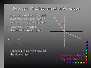
=. Refraction: What happens when V changes. In addition to being reflected at an interface, sound can be refracted, = change direction This refraction will be described by Snell’s Law: sin i 1 sin i 2 V 1 V 2 sound is always 'bent' toward the slower layer. i 1. V 1. V 2. i 2.

E N D
= Refraction: What happens when V changes • In addition to being reflected at an interface, sound can be refracted, = change direction • This refraction will be described by Snell’s Law: sin i1 sin i2 V1V2 • sound is always 'bent' toward the slower layer i1 V1 V2 i2 i1 = “angle of incidence” i2 = “angle of refractin”
Okay, so this is a bit juvenile • still, I like pictures!
Sound Velocity in water • Velocity increases with: • INcreasing pressure • INcreasing temperature • Velocity minimum at around 1,000m
The SOFAR Channel • Sound is bent toward the slower layer • this is always the center of the channel • sound is trapped
Shallow water acoustics • This only works if the water column is just right!
Refraction in Sediments • Sound is reflected from layers where acoustic impedence changes • Sound is refracted where velocity changes • These almost always co-occur
Refraction • This effect is of no consequence if the source and receiver are co-located • in order to ever receive the refracted signal, they have to be widely separated i1 V1 V2 i2
= Critical Refraction • If i1shallow enough, a neat thing happens: • i2 becomes 90o • this means that the sound arriving at this angle does not penetrate • instead it travels ALONG the interface • Snell’s law sin i1 sin 90o V1V2 i1 V1 V2 i2=90o
= Critical Refraction sin i1 sin 90o V1V2 i1 =sin-1 (V1/ V2) • We call the angle at which is occurs the “critical angle” • ic=sin-1 (V1/ V2) i1 V1 V2 i2=90o
An example* • Start with a layered bottom; discontinuity at 100m *Thanks to http://www.mines.edu
Watch the wave propagate: • both reflected and refracted returns
Resulting T vs. X Diagram Refracted
Refraction survey: T vs X plot • Must achieve xc • slopes of arrivals defined by in situ sound velocities • advantages: • velocity determination • deep penetration • disadvantages: • requires extra hardware • often two ships • need loud, low f sound source slope=1/v1 Time slope=1/vo xc Distance (x) Vo V1 Distance
Real World Example • with several layers, it gets more complicated • these are lines drawn by interpreter • actual arrival signals are far messier.
R2 F1 • to be more accurate, we need to show the curvature of these lines • note that a reflected arrival in one layer arrives at nearly the same time as the refracted from the next deeper layer (R2/F1) refracted arrival T reflected arrival direct water arrival X
A real-world example • VERY large scale
GRAVITY • gravity is used to determine: • Subsurface structures • Active tectonism • = another technique to determine subsurface features • a. local mass distributions • b. isostatic balance of an area. • gravimeter: mass on a series of springs • data are normally used in conjunction with other geophysical data • they are difficult (or impossible) to interpret alone and require several corrections:
Gravity • Gravity: Newton's law: F = G(m1m2) r2 where G=gravitational constant which is 6.67 x 10 dynes*cm /g • F = M x A (A is acceleration) = M1 x A • M1 x A = G(m1m2) (m1’s cancel) r2 • g = A = G x Me r2 • on earth, the acceleration is g=981mgals, • different on other planets • works only at earth’s surface
Gravity • The magnitude of measured gravity depends on 5 factors: • 1) latitude: • shape of the earth • rotation (centripidal force) • 2. elevation (r) • 3. topography • 4. Tides (solar and lunar positions) • 5. Presence and density of sub-surface mass • Because we’re interested in #5, we need to know and allow for all the other factors
Gravity: some notes • satellites fly along surfaces of equal gravitational potential • The geoid is a surface of equal potential which is approximated by mean sea level. • the geoid would be a sphere except that: • a. the earth is not a perfect sphere; equator is 43km larger diameter • b. anomalous deep-seated mass distributions within the earth,the geoid departs from the ideal by +70 to -100m • Our GEOID models correct for “all” of these effects • we use this reference to correct our measurements
GEOID Model • These heights are relative to a “suitable elipsoid”
Gravity: more notes • What happens to the GEOID if there is a buried mass? • the Geoid rises over masses local gravity is greater, so you have to go higher to achieve as constant value
Gravity notes • survey with instruments eg bubble level: • would actually tell you you're level relative to GEOID when it is NOT perpendicular to the earth's surface • "a ball would not roll on the geoid" • water surfaces define the geoid (almost)
Local mass variations affect measurements • true whether mass variation is “positive” or “negative” • here a buried mass affects the reading
Here a nearby mass affects the reading • ask your geodesy prof about how this correction is applied
Gravity • Corrections: as in much of science, you look for anomalies: • so you make all the corrections and then the difference between what you expect it to look like and what it actually looks like is called an anomaly. • 1. latitude correction: brings us to a known location on the reference spheroid. • This is a given; we also correct for tides, instrument calibration etc. at this step • the rest may or may not be done, depending on the goal of the project.
Gravity • 2. Elevation correction: • reduce to the elevation of the reference spheroid; • this accounts for the variations with r2 of gravitational attraction. • correct for the gradient of g in Air • gfreeair = 0.3086*h where h is the elevation (in meters) • This is called the Free Air correction • it’s subtracted from the measurement • what's left is called the "free-air anomaly" • Free air anomalies indicate: • a. buried masses • b. isostatic disequilibrium
Gravity • 3. Bouger correction: corrects for the density of material between the gravity station and the reference surface. • at sea reference is the sea floor • on land reference is sea level • these two meet at coast • gBouger = 0.04185rh • h is the thickness of the layer you are trying to compensate for (water or rock) • r is the density of that layer; • need to know what kind of rock is there • Flat, elevated areas above sea level characteristically have large negative Bouger anomalies, • Ocean basins have large positive Bouger anomalies • gfreeair - gBouger = Bouger anomaly • may also apply a “terrain correction”
Gravity • Isostasy: Bouger anomalies compensate for the density of rocks between the station and the reference surface only. • You find negative anomalies over the continents and positive anomalies over the oceans. • But, crustal masses are like icebergs floating on the mantle, they have deep roots. • If you look at the depth to the mantle and apply this "isostatic correction", you get the isostatic anomaly.
The pressure is the same at all places because the wood weighs the same as the water it displaces
The extra mass (the mountain) forces a depresession in the Moho
Gravity • In the geological application, elevated areas have deep expression • the crust is thicker in these places • if you compare the gravity there, you get lower than expected values because the integrated mass is less
Crustal Thicknesses • P wave velocities • Layer 1 = sediments • 1.6-2.5km/sec • Layer 2 = Basalt • 5-6km/sec (pillows) • 6-7km/sec (dikes) • Layer 3= Gabbro • 7km/sec • Continental crust is thicker than oceanic crust. • Note: • Seychelles • Ontong Java • Iceland
Gravity • To compensate for “mountain roots”, we need to know how deep they extend and what their mass is • The depth is = depth to the Moho (crustal thickness) • Crustal density is pretty uniform, so we use a generic number • Note that you need geophysical data (depth to the Moho) in order to make this correction!! • What's left is the Isostatic Anomaly and it indicates places which are out of isostatic equilibrium. • clearly the most interesting of anomalies • but most difficult to produce • Where Isostatic Anomaly is zero, no activity is present • Where it’s positive or negative, plates are on the move!
Gravity • Isostatic anomaly = Observed + latitude correction + altitude correction (Free air correction) + Bouger correction + terrain correction + tide correction + Isostatic correction • Most of the earth is in reasonable isostatic equilibrium, • ie the masses of the mountains are compensated for by low density roots, • the basins are low due to the high density and small thickness of oceanic crust. • However anomalies do exist. Bouger Land surface Isostatic Free air
Gravity • Places to find isostatic anomalies • 1. places where ice sheets have recently receded are rebounding • 300m in last 10,000 years!!! • Remember, this was a LOT of ice!
2. active tectonism • trenches • mid ocean ridges • other faulting areas
Even the continental US still has some surprising gravity anomalies!