Download
1 / 22
220 likes | 291 Views
Using Parcel Level Data for an Activity-Based Tour Model. TRB Transportation Planning Application Conference May 8, 2007. Background for Modeling. Long Range Land Use “Blueprint” “4 D’s” emphasis Regionally adopted In process of developing first Blueprint transportation plan

E N D
Using Parcel Level Data for an Activity-Based Tour Model TRB Transportation Planning Application Conference May 8, 2007
Background for Modeling • Long Range Land Use “Blueprint” • “4 D’s” emphasis • Regionally adopted • In process of developing first Blueprint transportation plan • Place3s Land Use Scenario/Analysis Tool • “Parcel” level data • Place type
Background for Modeling (cont’d) • Limitations of zone-based model • Many 4 D’s factors missed by zone aggregation • Developed SACSIM (Activity-Based Tour Model) • Familiar model (similar to SF, others) • Based on parcel-level land use data • Motorized Networks still TAZ-based for assignment • Skims combine TAZ skims and direct parcel/point proximity measures
Types of Parcel/Point Data Files • Place3s “Parcel” Files • Place Type, Acres • # Dwellings • # Jobs • Schools • K12 (all types) • College/University • 4+ year colleges • Community colleges • Paid Off-Street Parking • # Spaces • $ / day, $ / hour
Types of Parcel/Point Data Files (cont’d) • Street Pattern • Intersection points by type • Types = 1, 3, 4+ legs / node • Transit stations/stops • LRT, rail stations • Fixed route bus stops • Park-and-ride facilities
Parcel/Point Data Formulations • Point values • # of dwellings, jobs, school enrollments, etc. at the parcel/point • Buffered point values • # of dwellings, jobs, etc. within ¼ or ½ mile of parcel
Strategies for Developing Datasets • Yield Estimation for Land Use Scenario • Qi = acrespt x yieldi • Used for both “base year” (2005) and future year dataset • Future year land use scenarios developed in Place3s • Inventory + Change • Base year points from inventory • Future year change from other source (Place3s, travel model networks, etc.)
Examples of Inventory+Change Approach • Street Pattern / Intersection Density • Use actual GIS intersection points for 2005 • For future year, use Place3s comparisons between 2005 and future year to identify “change” parcels • Apply lookup rates by place type to change parcels
Examples of Inventory+Change Approach (cont’d) • Transit stops • Use 2005 GIS inventory of stops for base year • Identify new lines by comparing 2005 and future year travel model transit networks (zone-base) • Synthesize transit stops for the new lines • Add new stops to inventory
Scale of Data Production • Place3s land use datasets are the basis • Separate staff to work with local agencies, committees etc. to develop land use scenarios in Place3s • 2 persons full-time, 4-5 part time dedicated to this effort • Place3s used for many land use planning, outreach and public relations functions
Scale of Data Production (cont’d) • Inventory Data • Housing, employment, schools, transit stops • Separate function, 5-6 staff work part time on this • Episodic (updates every 2-3 years or for special projects
Scale of Data Production (cont’d) • Time required to generate a full SACSIM dataset • Starting point: Complete, regional Place3s dataset • Ending point: Complete, runnable SACSIM dataset • Approximate duration: 1-2 weeks • Approximate staff time: 50 hours, spread between 4 staff • 20-30 hours running time for buffering a new file (single thread workstation)
Making It Faster • Buffering: selective re-buffering • Up front QC of files • Re-do’s are painful… • Multi-threading / server farm (in budget next year)
Acknowledgments • ABTM Model (Daysim) Designers, Architects • John Bowman, Ph.D • Mark Bradley • Application and Shell Program Developers • John Gibb, DKS Associates • Parcel Data Production Process • Steve Hossack, SACOG