Download

1 / 40
400 likes | 421 Views
This document provides an overview of the χ2 and Goodness of Fit methods for straight line fitting, including the concepts of σ, correlated errors, and the determination of parameters. It also discusses the limitations and considerations of the least squares method, as well as alternative methods for assessing the goodness of fit. The document is based on the work by Louis Lyons and Lorenzo Moneta from Imperial College and Oxford, presented at CERN IPMU in March 2017.

E N D
χ2 and Goodness of Fit Louis Lyons andLorenzo Moneta Imperial College & Oxford CERN IPMU March 2017
Least squares best fit What is σ? Resume of straight line Correlated errors Goodness of fit with χ2 Number of Degrees of Freedom Other G of F methods Errors of First and Second Kind Combinations THE paradox
Least Squares Straight Line Fitting Data = {xi, yi ±δyi} • Does it fit straight line? • (Goodness of Fit) • 2) What are gradient and intercept? • (Parameter Determination) • Do 2) first • N.B.1 Can be used for non “a+bx” • e.g. a + b/x + c/x2 • N.B.2 Least squares is not the only method (Goodness of Fit)
If theory and data OK: yth ~ yobs S small Minimise S best line Value of Smin how good fit is
Which σ should we use? Which σ? Exptl σ Theory σ Name Neyman Pearson Ease of algebra Easier, so this version is used more If Th = 0.01, Exp = 1 Contributes 1 to S Contributes 98 to S More plausible S ~ χ2 ? More plausible S = (â-a1)2/σ12 + Biassed down because Biassed up because (â -a2)2/σ22 smaller ai smaller σ larger â larger σ (For â ~ai, and both much larger than σi, 2 methods are very similar)
Straight Line Fit (Fixed σi ) <y> N.B. L.S.B.F. passes through (<x>, <y>)
Correlated intercept and gradient? 2 * Inverse covariance matrix = ∂2S ∂2S Σ1/σi2Σxi/σi2 ∂a2 ∂a∂b = ∂2S ∂2S Σxi/σi2Σxi2/σi2 ∂a∂b ∂b2 Invert Covariance matrix Covariance ~ -Σxi/σi2 = [x] If measure intercept at weighted c. of g. of x for data points, cov = 0 i.e. gradient and intercept there are uncorrelated So track params are usually specified at centre of track.
Covariance(a,b) ~ -<x> <x> positive <x> negative b y a x
Comments on Least Squares method 1) Need to bin Beware of too few events/bin 2) Extends to n dimensions but needs lots of events for n larger than 2 or 3 3) No problem with correlated uncertainties 4) Can calculate Smin “on line” i.e. single pass through data Σ (yi – a –bxi)2 /σ2 = [yi2] – b [xiyi] –a [yi] 5) For theory linear in params, analytic solution y 6) Goodness of Fit x
Goodness of Fit: χ2test • Construct S and minimise wrt free parameters • Determine ν = no. of degrees of freedom ν = n – p n = no. of data points p = no. of FREE parameters • Look up probability that,forν degrees of freedom, χ2 ≥ Smin Uses i) Poisson ~ Gaussian if expected number not too small ii) For N yi distributed as Gaussian N(0,1), Σyi2 ~ χ2 with ndf = N So works ASYMPTOTICALLY. Otherwise use MC for dist of S (or binned L)
Properties of mathematical χ2 distribution: χ2= ν σ2(χ2) = 2ν So Smin > ν + 3√2ν is LARGE e.g. Smin = 2200 for ν = 2000?
χ2 with ν degrees of freedom? ν = data – free parameters ? Why asymptotic (apart from Poisson Gaussian) ? a) Fit flatish histogram with y = N {1 + 10-6 cos(x-x0)} x0 = free param b) Neutrino oscillations: almost degenerate parameters y ~ 1 – A sin2(1.27 Δm2 L/E) 2 parameters 1 – A (1.27 Δm2 L/E)2 1 parameter Small Δm2
Goodness of Fit . χ2 Very general Needs binning Not sensitive to sign of deviation Run Test Kolmogorov-Smirnov Aslan and Zech `Energy Test’ Durham IPPP Stats Conf (2002) Binned Likelihood ( = Baker-Cousins} etc
Goodness of Fit: Kolmogorov-Smirnov Compares data and model cumulative plots (or 2 sets of data) Uses largest discrepancy between dists. Model can be analytic or MC sample Uses individual data points Not so sensitive to deviations in tails (so variants of K-S exist) Not readily extendible to more dimensions Distribution-free conversion to p; depends on n (but not when free parameters involved – needs MC)
Goodness of fit: ‘Energy’ test Assign +ve charge to data ; -ve charge to M.C. Calculate ‘electrostatic energy E’ of charges If distributions agree, E ~ 0 If distributions don’t overlap, E is positive v2 Assess significance of magnitude of E by MC N.B. v1 • Works in many dimensions • Needs metric for each variable (make variances similar?) • E ~ Σ qiqj f(Δr = |ri – rj|) , f = 1/(Δr + ε) or –ln(Δr + ε) Performance insensitive to choice of small ε See Aslan and Zech’s paper at: http://www.ippp.dur.ac.uk/Workshops/02/statistics/program.shtml
Binned data and Goodness of Fit using L-ratio For histogram, uses Poisson prob P(n;µ) for n ni observed events when expect µ. Construct L-ratio = Product{P(ni;µi)/P(ni;µ=ni)} P(ni;µ=ni) is best possible µ for that ni µi Need denoms because P(100;100.0) very different from P(1;1.0) x -2*L ratio ~ χ2 when µi large and ni ~ µi Better than Neyman or Pearson χ2when µi small Baker and Cousins, NIM 221 (1984) 437
Wrong Decisions Error of First Kind Reject H0 when true Should happen x% of tests Errors of Second Kind Accept H0 when something else is true Frequency depends on ……… i) How similar other hypotheses are e.g. H0 = μ Alternatives are: e π K p ii) Relative frequencies: 10-4 10-4 1 0.1 0.1 Aim for maximum efficiency Low error of 1st kind maximum purity Low error of 2nd kind As χ2 cut tightens, efficiency and purity Choose compromise
How serious are errors of 1st and 2nd kind? • Result of experiment e.g Is spin of resonance = 2? Get answer WRONG Where to set cut? Small cut Reject when correct Large cut Never reject anything Depends on nature of H0 e.g. Does answer agree with previous expt? Is expt consistent with special relativity? 2) Class selector e.g. b-quark / galaxy type / γ-induced cosmic shower Error of 1st kind: Loss of efficiency Error of 2nd kind: More background Usually easier to allow for 1st than for 2nd 3) Track finding
Combining: Uncorrelated exptl results Simple Example of Minimising S N.B. Better to combine data rather than results So â = Σwiai/Σwi , where wi=1/σi2
Difference between weighted and simple averaging Isolated island with conservative inhabitants How many married people ? Number of married men = 100 ± 5 K Number of married women = 80 ± 30 K Total = 180 ± 30 K Wtd average = 99 ± 5 K CONTRAST Total = 198 ± 10 K GENERAL POINT: Adding (uncontroversial) theoretical input can improve precision of answer Compare “kinematic fitting”
BLUEBest Linear UnbiassedEstimate Combine several possibly correlated estimates of same quantity e.g. v1, v2, v3 Covariance matrix σ12cov12 cov13 cov12σ22 cov23 cov13 cov23σ32 Uncorrelated Positive correlation Negative correlation covij = ρijσiσj with -1 ≤ ρ ≤ 1 Lyons, Gibault + Clifford NIM A270 (1988) 42
vbest = w1v1 + w2v2 + w3v3Linear with w1 + w2 + w3 =1 Unbiassed to give σbest = min (wrt w1, w2, w3) Best For uncorrelated case, wi~ 1/σi2 For correlated pair of measurements with σ1 < σ2 vbest = α v1 + β v2 β = 1 - α β = 0 for ρ= σ1/σ2 β < 0 for ρ > σ1/σ2 i.e. extrapolation! e.g. vbest = 2v1 – v2 Extrapolation is sensible: V Vtrue v1 v2
Beware extrapolations because [b] σbest tends to zero, for ρ = +1 or -1 [a] vbest sensitive to ρ and σ1/σ2 N.B. For different analyses of ~ same data, ρ ~ 1, so choose ‘better’ analysis, rather than combining
N.B. σbest depends on σ1, σ2 and ρ, but not on v1 – v2 e.g. Combining 0±3 and x±3 gives x/2 ± 2 BLUE = χ2 S(vbest) = Σ (vi – vbest) E-1ij (vj – vbest) , and minimise S wrt vbest Smin distributed like χ2, so measures Goodness of Fit But BLUE gives weights for each vi Can be used to see contributions to σbest from each source of uncertainties e.g. statistical and systematics different systematics For combining two or more possibly correlated measured quantities {e.g. intercepts and gradients of a straight line), use χ2 approach. Alternatively. Valassi has extended BLUE approach
Covariance(a,b) ~ -<x> <x> positive <x> negative b y a x
Uncertainty on Ωdark energy When combining pairs of variables, the uncertainties on the combined parameters can be much smaller than any of theindividualuncertainties e.g. Ωdark energy
THE PARADOX Histogram with 100 bins Fit with 1 parameter Smin: χ2 with NDF = 99 (Expected χ2 = 99 ± 14) For our data, Smin(p0) = 90 Is p2 acceptable if S(p2) = 115? YES. Very acceptable χ2 probability NO. σp from S(p0 +σp) = Smin +1 = 91 But S(p2) – S(p0) = 25 So p2 is 5σ away from best value
Next time: Bayes and Frequentism: the return of an old controversy The ideologies, with examples Upper limits Feldman and Cousins Summary
KINEMATIC FITTING Tests whether observed event is consistent with specified reaction
Kinematic Fitting: Why do it? • Check whether event consistent with hypothesis [Goodness of Fit] • 2) Can calculate missing quantities [Paramdetn.] • 3) Good to have tracks conserving E-P [Paramdetn.] • 4) Reduces uncertainties [Paramdetn.]
Kinematic Fitting: Why do it? • Check whether event consistent with hypothesis [Goodness of Fit] • Use Smin and ndf • 2) Can calculate missing quantities [Paramdetn.] • e.g. Can obtain |P| for short/straight track, neutral beam; px,py,pz of outgoing ν, n, K0 • 3) Good to have tracks conserving E-P [Paramdetn.] • e.g. identical values for resonance mass from prodn or decay • 4) Reduces uncertainties [Paramdetn.] • Example of “Including theoretical input reduces uncertainties”
How we perform Kinematic Fitting ? Observed event: 4 outgoing charged tracks Assumed reaction: ppppπ+π- Measured variables: 4-momenta of each track, vimeas (i.e. 3-momenta & assumed mass) Then test hypothesis: Observed event = example of assumed reaction i.e. Can tracks be wiggled “a bit” to do so? Tested by: Smin = Σ(vifitted- vimeas)2 / σ2 where vifittedconserve 4-momenta (Σ over 4 components of each track) N.B. Really need to take correlations into account i.e. Minimisation subject to constraints (involves Lagrange Multipliers)
‘KINEMATIC’ FITTING Angles of triangle: θ1 + θ2 + θ3 = 180 θ1θ2θ3 Measured 50 60 73±1 Sum = 183 Fitted 49 59 72 180 χ2 = (50-49)2/12 + 1 + 1 =3 Prob {χ21 > 3} =8.3% ALTERNATIVELY: Sum =183 ± 1.7, while expect 180 Prob{Gaussian 2-tail area beyond 1.73σ} = 8.3%