Download
1 / 50
510 likes | 687 Views
Observation of radiation belt losses into the ionosphere. Craig J. Rodger Department of Physics University of Otago Dunedin NEW ZEALAND. REPW 2007 2:45pm Wednesday, 8 August 2007. Energetic electrons, the Radiation Belts, and Geomagnetic Storms.

E N D
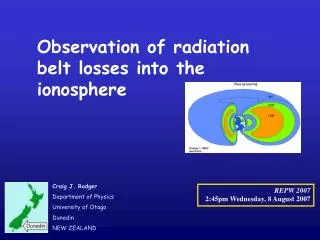
Observation of radiation belt losses into the ionosphere Craig J. Rodger Department of Physics University of Otago Dunedin NEW ZEALAND REPW 2007 2:45pm Wednesday, 8 August 2007
Energetic electrons, the Radiation Belts, and Geomagnetic Storms Losses:overall response of the RB to geomagnetic storms are a "delicate and complicated balance between the effects of particle acceleration and loss". [Reeves et al., GRL, 2003]. Essentially all geomagnetic storms substantially alter the electron radiation belt populations, and losses play a major role. A significant fraction of the particles are lost into the atmosphere, although storm-time non-adiabatic magnetic field changes also led to losses through magnetopause shadowing (particularly during storm-times). In today's talk I want to discuss some studies we have done on particle precipitation from the RB:during storms (FAST and SLOW events)after storms
Energetic Precipitation from the RB affects the lower ionosphere For electrons >100keV, the bulk of the precipitated energy is deposited into the middle and upper atmosphere (30-100km), and can be detected through changes in subionospheric VLF propagation. REP Subionospheric VLF signals reflect from the ionospheric D-region. →received radio waves are largely determined by propagation between the boundaries→ Very-long range remote sensing is possible (1000's of km )!
For frequencies >10 kHz man-made transmissions from communication and navigation transmitters can be observed in almost every part of the world, as seen in the spectra below. Very-long range remote sensing is possible as the transmitter signals can be received 1000's of km from their sources! South Africa New Zealand Israel Antarctica
Our AARDDVARK An aarmory of AARDDVARKs. This map shows our existing network of sub-ionospheric energetic precipitation monitors. MORE INFORMATION: www.physics.otago.ac.nz\space\AARDDVARK_homepage.htm
Part I: FASTREP • Part I is based on the following publication: Rodger, C. J., M. A. Clilverd, D. Nunn, P. T. Verronen, J. Bortnik, and E. Turunen, Storm-time short-lived bursts of relativistic electron precipitation detected by subionospheric radio wave propagation, J. Geophys. Res., 112, A07301, doi:10.1029/2007JA012347, 2007.
Microbursts These pulses here! RELATIVISTIC MICROBUSRTS • >1 MeV microbursts lasting <<1 s (L=4-6) • typically observed at the outer edge of the radiation belt • observed at all local times, but occur predominantly in the morning sector • Thought to be associated with VLF chorus waves [Lorentzen et al., 2001] SAMPEX satellite observed fluxes show that microburst precipitation losses can essentially "flush out" the entire relativistic electron population during the main phase of the storm. However, the global loss estimates are based upon the assumption that the microburst flux is isotropic and constant over selected L and MLT ranges. Ground based observations would complement the space-based point measurements! FAST Process!
REP Microbursts The distinction between relativistic and non-relativistic microbursts is an important one. Non-relativistic microbursts have been known of for some time: Non-relativistic (>150 keV) microbursts are also of short duration (~0.2-0.3 s), and occur on the dayside. Rocket and balloon measurements indicate that the precipitating electrons are primarily in the tens to hundreds of keV range, with negligible fluxes above 1 MeV. SAMPEX observations have also shown that REP microbursts are often accompanied by non-relativistic (>150 keV) microbursts, but the bursts in the two energy channels do not exhibit a one-to-one correspondence. So REP microbursts and non-REP microbursts can occur in the same time periods and rough locations, but are very unlikely to be created simultaneously through the same process.
REP Microbursts & Chorus REP microbursts are correlated with satellite observed VLF chorus wave activity: * short duration of microbursts similar chorus elements *similarity in LT distributions have lead to the widely held assumption that REP microbursts are produced by wave-particle interactions with chorus waves. However, this has yet to be confirmed, and a one-to-one correlation of REP microbursts and chorus elements has yet to be demonstrated. Here we examine ground-based ionospheric data during REP activity to better understand the energy spectra and hence the source mechanism Chorus observed in Dunedin on 7 Feb 2005
We start by focussing on the late January 2005 period. This was a fairly disturbed time, with numerous solar flares (X-rays striking the upper atmosphere). A fairly large solar flare on 20 January 2005 produced an unusually hard SPE (protons striking the upper atmosphere). An associated CME triggered a geomagnetic storm, leading to a relativistic electron drop-out on 21 Jan 2005.
Observation setup During 21 January 2005 (and also 4 April 2005) our subionospheric VLF receivers were operating at several different locations, observing transmitters that span a wide range of longitude sectors and L-shells.
REP observed at SGO on 21 Jan 2005 Summary Plot. Amplitude subionospheric VLF observations at 17-18UT from SGO. FAST losses on top of the SLOW losses. NOTE: There appears to be two different time scales seen in this data – changes on ~5min timescales and also short lived spikes, which is what I want to focus on first.
REP observed at SGO on 21 Jan 2005 Different Summary Plot. Period which emphasizes the FAST subionospheric amplitude perturbations observed on multiple transmitters at SGO.
Examples of FASTREP in SGO data The residual amplitudes that remain after removing the smoothed background with a 5s filter, drawing out the rapid changes. Shows many large short-lived spike events of 1-5 dB, both increases and decreases. Similar short lived large negative and positive perturbations are also observed in the transmitter phase. Almost certainly the first ground-based observations of relativistic electron microbursts.
Examples of FASTREP in SGO data Over the 4 hour period 17-21 UT, 221 FAST perturbations were observed on transmissions from NAA and 109 on NDK, i.e. a rough rate of 1 per minute on each GCP. The majority of the FAST perturbations are not simultaneous with perturbations on other paths even though they occur during the same periods. However, a very small fraction, on the order of ~1-2% appear to be simultaneous on multiple paths. This behaviour is consistent with ionospheric changes with small spatial size, occurring near to the Sodankylä receiver. A useful analogy is a rainstorm, with many small raindrops, each representing a burst of precipitating electrons, produced by the same physical process spanning a much larger spatial region.
Timescales of FASTREP 60s worth of Sodankylä-received subionospheric amplitude from VLF transmitters on 21 January 2005, plotted at the maximum 0.1s time resolution. Several well defined FAST features are evident, each lasting roughly ~1 s, as well as a feature on NDK lasting ~6 s which appears to be made up of multiple discrete pulses. The well defined FAST features are typical for the short-lived pulses seen on 21 January 2005, made up of a 0.2 s rise followed by a 0.5 s decay to background amplitude levels.
Timescales of FASTREP Another example, this time on NDK. Generally a ~0.2s risetime, following by a ~0.5s decay, but with some events appearing to be made up of multiple events. The rapid decay time is highly suggestive of a short-lived highly energetic precipitation burst producing significant additional ionization at ~60km altitude (peak ionization altitude for a ~1.5MeV electron). We therefore conclude that the FAST subionospheric VLF perturbations are most consistent with the ionization signature caused by REP microbursts. Time resolution:0.1 s points
REP precipitation on 3 April 2005 Fundamentally similar to the perturbations observed on 21 Jan 2005, the decay time of these events are a factor of ~3 longer (1.4 s c.f. 0.5 s), consistent with masking of higher altitude ionization changes from subionospheric detection due to the proton precipitation continuing on from the 20 Jan 2005 SPE. This provides strong evidence that that the FASTREP is produced by short-lived bursts of REP, with the "real" perturbation-decay time being ~1.5 s when unmasked by ionization produced from other precipitation.
Modelling of Chorus produced VLF perturbations It is widely assumed in the community that REP microbursts are due to chorus waves. In order to test the REP microburst observations against the expected signature for chorus produced precipitation, we make use of calculated precipitation fluxes produced by a single chorus element at L=5 at 100km altitude. The chorus rays are launched from the geomagnetic equator . As these rays propagate, they resonate with counter-streaming energetic electrons through the m=1 resonance mode.
Modelling of Chorus produced VLF perturbations N. Hemisphere S. Hemisphere However, because these chorus waves are oblique, higher order resonances are also possible, including both counter- and co-streaming orientations. The calculation is undertaken using a test-particle simulation assuming AE-8 trapped electron flux levels, and an isotropic distribution that is sharply cutoff at the loss cone. N. hemisphere: 2 energy groupings, ~4-30keV & ~150 keV-4MeV S. Hemisphere: single high energy grouping, spanning ~50keV-3MeV
Effect of precipitation on atmosphere Assume northern hemisphere chorus precipitation pattern (but it doesn’t matter for D-region) To describe the atmospheric impact of the chorus-produced precipitation, we make use of the Sodankylä Ion Chemistry model. The SIC model runs were undertaken for polar night conditions appropriate for 17 UT on 21 Jan 2005 at a location of (69ºN, 22.5ºE), i.e., close to our receiver in Finland. This figure shows the time varying electron number density profiles determined from the SIC model.
Modelled VLF perturbation from chorus REP 21:36:54.80 UT, 5 April 2005 100’s keV precipitating electrons make long-lasting ionospheric modification >70 km and hence negative amplitude perturbation. Apply the SIC-determined electron densities to the VLF propagation code Modefinder and see what the perturbation looks like. It does not do a very good job of reproducing the FAST VLF signature – too much low energy electrons present which impact at high altitudes.
Modelled VLF perturbation from mono-energetic REP beams 21:36:54.80 UT, 5 April 2005 Try 0.1s monoenergetic beams with flux of 100 el.cm-2s-1sr-1 (similar to SAMPEX) and contrast with the same microburst decay time. We need a highly energetic beam with no significant electron flux less than ~1.5MeV to reproduce the decay time of our VLF perturbations. This is not consistent with chorus production, but is consistent with the satellite observations of relativistic REP microbursts.
Summary - Part I • On 21 January 2005 a relativistic electron drop-out at GEO was associated with several hundred short-lived VLF perturbations observed by the AARDDVARK receiver at SGO over ~4 hours. • The vast majority of these perturbations were not simultaneous with perturbations on other nearby paths precipitation "rainstorm" producing ionospheric changes of small spatial sizes around the Sodankylä receiver. • 1.5s VLF perturbation decay time is consistent with short-lived bursts of REP, observed by satellites as relativistic microbursts. To the best of the authors knowledge, this is the first ground based observation of microburst REP. • Contrasts between predicted VLF perturbations for chorus driven precipitation, and those due to more highly energetic beams indicate that the recovery time is most consistent with precipitation containing only highly relativistic populations, principally from energies greater than about 2 MeV. • The chorus-driven VLF perturbations were very unlike the experimentally observed VLF perturbations, and unlike the reported energy spectra of satellite observed relativistic microbursts.
Part II: REPJGR • Part II is based on the following publication: Clilverd, M. A., C. J. Rodger, R. M. Millan, J. G. Sample, M. Kokorowski, M. P. McCarthy, Th. Ulich, T. Raita, A. J. Kavanagh, and E. Spanswick, Energetic particle precipitation into the middle atmosphere triggered by a coronal mass ejection, J. Geophys. Res., (in press), 2007.
Minutes-to-hours MeV precipitation MeV Precipitation • >0.5 MeV precipitation lasting minutes-hours • Located between L=3.8-6.7 • observed only in the late afternoon/dusk sector (14:30-00:00 MLT) • May be produced by EMIC waves [Millan et al., 2002] MAXIS balloon observed fluxes show that this precipitation mechanism is a primary loss process for outer zone relativistic electrons. Plot taken from: Millan, R. M., R. P. Lin, D. M. Smith, K. R. Lorentzen, and M. P. McCarthy, X-ray observations of MeV electron precipitation with a balloon-borne germanium spectrometer, Geophys. Res. Lett., 29(24), 2194, doi:10.1029/2002GL015922, 2002. SLOW Process!
Initial conditions - CME impact ACE ACE data is delayed to reflect expected CME arrival time. 17.2 = 17:10 UT ACE GOES
In Jan 2005 MINIS balloons were launched through the AARDDVARK network
Dusk Sector ~20 MLT Scandinavia L= 5-6 Riometer + VLF (Iceland – SGO) L= 2.5-4 Riometer + VLF (Germany – SGO) + Pulsation mags
Dusk Sector Initial pulse L= 5-6 Riometer + VLF (Iceland – SGO) Initial pulse L= 2.5-4 Riometer + VLF (Germany – SGO) Extended precipitation
Prolonged precipitation for ~1 hour 4 November 2003 Thomson’s Great Flare (X45) Peak flux ~17.3-17.35 UT
Nurmijarvi Pulsation Magnetometer EMIC band L=3.4
IMAGE EUV observation of plasmasphere Compressed plasmasphere ~5 hours after CME, with Kp=8 SUN The position of the plasmapause is consistent with EMIC-induced precipitation of electrons at L=2-3 Lpp ~ 2-3
Dayside~10-15 MLTNorthern H >30 keV Using Walt [1994] to calculate an azimuthal drift period at L=4.0 14 mins = 1.5 MeV 17 mins = 0.8 MeV 14 mins >100 keV 17 mins
Halley- Dayside~10-15 MLTSouthern H >100 keV Some bursty precipitation events, although the timing is not clearly linked to the northern hemisphere events, apart from Flt3S L=4.1 Some interesting comparisons between MINIS balloon X-ray counts and riometer data >30 keV >20 keV -10 MeV
Map of precipitation Initial arrival of the CME causes precipitation over L from ~3-8, and probably over all MLT. (initial burst also seen by Macquarie Island riometer. Nothing in Dunedin-Australian VLF data, hence lower cutoff). The nightside precipitation is more localised, and the dayside rather bursty.
Summary: Part II • Detectable levels of energetic precipitation into the atmosphere following the 21 January 2005 CME. • Initial precipitation lasting ~ 5 minutes, observed over a large proportion of the Earth. • Dayside precipitation bursty and suggests drifting electrons ~1 MeV interacting with a loss region at L=4. • Duskside precipitation appears to be associated with the location of the plasmapause and produced by EMIC waves, which were simultaneously recorded in southern Finland. • We are now working to increase our database of EMIC waves with similar events, and work on the precipitation fluxes and energy spectrum.
Part III: CRRESREP • Part III is based on the following publication: Rodger, C. J., M. A. Clilverd, N. R. Thomson, R. J. Gamble, A. Seppälä, E. Turunen, N. P. Meredith, M. Parrot, J. A. Sauvaud, and J.-J. Berthelier, Radiation belt electron precipitation into the atmosphere: recovery from a geomagnetic storm, J. Geophys. Res., (in press), 2007.
Proton fluxes DEMETER measured drift-loss cone electron fluxes at L=3.2 Dst Geomagnetic storm of 11 Sept 2005 led to an increase in the energetic electron population in the inner edge of the outer radiation belt 1000 times ambient 100 above pre-storm levels decays over ~14 days to pre-storm levels (and 5 times above ambient), after which there is a DEMETER data-gap Kp
DEMETER: 128 energy channels (70keV-2.34 MeV) CRRES 17 energy channels (153keV -1.582 MeV) NOTE: CRRES shifted to fit DEMETER fluxes Hardening in electron spectra seen by the low-Earth orbiting DEMETER in drift-loss cone is consistent with that seen by CRRES near the geomagnetic equator in June 1991. We represent the spectra by the fitted power law shown.
Subionospheric Observations NYA, Ny Ålesund SGO, Sodankylä CAM, Cambridge NAA, 24kHz 600kW From 1 September 2005 we undertook subionospheric observations of NAA from our 3 European AARDDVARK receiver sites.
Dominated by Solar Proton Event line = SPE Mid L=12 Solar Proton Event and something else? Mid L=7.5 Undisturbed level Must be precipitation from RB (too low L for protons) Mid L=3.2 Change in NAA at CAM due to energetic electron precipitation: 14±1 dB decrease at Midnight 2.4±0.3 dB increase at Midday
Model the ionospheric changes >150keV electron flux: 200 el. cm-2 s-1 • Sweep through range of precip. fluxes • Use a simplified ionospheric chemistry scheme to determine the D-region electron density after precipitation (checked by the Sodankylä Ion Chemistry Model) • Use this as an input for the subionospheric propagation code LWPC HENCE predict expected change in amplitude for a given precipitation along our NAA-CAM path.
Subionospheric measurements of precip. Precipitation fluxes required to reproduce the changes in subionospheric propagation observed (NAA -> CAM). Peak Fluxes: 3500±300 el. cm-2s-1 at midday 185±15 el. cm-2s-1 at midnight. NOTE: after storm, day fluxes are ~20 times higher than night fluxes (for 6 days). This is consistent with plasmaspheric hiss observations. During geomagnetically disturbed conditions (AE*>150 nT) CRRES found 0.2-0.5kHz hiss was ~10 times stronger on dayside than nightside. With DEMETER wave-data we can test this!
DEMETER observations of plasmaspheric hiss • At L=3.2 resonance: 0.5 kHz waves with 160keV electrons~40 Hz waves with 1 MeV electrons • Use DEMETER to look at this wave range and L-range above our transmitter-receiver Great Circle Path. • Both wave and particles show a factor ~200 increase during 9-11 Sept. • Daytime wave powers ~10 times nighttime in post-storm period, much like seen in the precipitating particle measurements. Dawnside equatorial chorus does not reproduce the day-night differences seen in our precipitation fluxes, as it has peak intensities on the morning and evening sides. Off-equatorial chorus is 100 times stronger on day than night.
Summary - Part III After 11 September 2005 geomagnetic storm the >150 keV electron fluxes in the drift loss cone at L=3.2 increased by a factor of ~1000 above ambient conditions. The fluxes decayed to within a factor of 5 of the ambient levels over the following 14 days. Measured energy spectrum is consistent with previous observations of storm-time flux increases. Subionospheric VLF measurements allow us to quantify the precipitation losses, effectively "resolving" the bounce loss cone. The peak precipitated fluxes of >150 keV electrons into the atmosphere were 3500±300 el. cm-2s-1 at midday and 185±15 el. cm-2s-1 at midnight. Plasmaspheric hiss (PH) observations show reasonable agreement with precipitating particle behaviour, suggesting PH with freqs <500 Hz primary driver of energetic electron losses outside storm periods.
Conclusions The precipitation of energetic radiation belt particles can be detected from the ionosphere, providing a complementary way of looking at these events. We have advanced our tools a great deal, and are now able to provide indications of precipitating flux in many situations. The AARDDVARK network is well positioned to work alongside upcoming missions, like DSX, RBSP and ORBITALS.
1st international HEPPA Workshop 2008"High-Energy Particle Precipitation in the Atmosphere" 28-31 May 2008 Finnish Meteorological Institute, Helsinki, Finland Focus: Observations and modelling of atmospheric and ionospheric changes caused by energetic particle precipitation, e.g. solar proton events, relativistic electron precipitation, and auroral electron precipitation. Topics ranging from short-term ionospheric changes to long-term atmospheric changes are welcome, including defining spectra of precipitating particles and the effects on atmospheric dynamics. http://heppa2008.fmi.fi Registration begins in October 2007
Craig visiting the Artillery Museum. St. Petersburg, October 2006 Thankyou! Are there any questions?

![[The Virtual Radiation Belt Observatory]](https://cdn2.slideserve.com/5073406/the-virtual-radiation-belt-observatory-dt.jpg)

![[The Virtual Radiation Belt Observatory]](https://cdn5.slideserve.com/9698782/the-virtual-radiation-belt-observatory-dt.jpg)