Answering Distance Queries in directed graphs using fast matrix multiplication

1. Answering Distance Queries in directed graphs using fast matrix multiplication Seminar in Algorithms Prof. Haim Kaplan Lecture by Lior Eldar 1/07/2007

2. Structure of Lecture • Introduction & History • Alg1 – APSP • Alg2 – preprocess & query • Alg3 – Hybrid • Summary

3. Problem Definition • Given a weighted directed graph, we are requested to find: • APSP - All pairs shortest paths – find for any pair • SSSP - Single Source shortest paths – find all distances from s. • A hybrid problem comes to mind: • Preprocess the graph faster than APSP • Answer ANY two-node distance query faster than SSSP. • What’s it good for?

4. Previously known results – APSP • Undirected graphs • Approximated algorithm by Thorup and Zwick: • Preprocess undirected weighted graph in expected time. • Generate data structure of size • Answer any query in O(1) • BUT: answer is approximate with a factor of 2k-1. • For non-negative integer weights at most M – Shoshan and Zwick developed an algorithm of run time • Directed graphs – Zwick - runs in

5. Previously known results - SSSP • Positive weights: • Directed graphs with positive weights – Dijkstra with • Undirected graphs with positive integer edge weights – Thorup with • Negative weights – much harder: • Bellman-Ford • Goldberg and Tarjan – assumes edge weight values are at least – N.

6. New Algorithm by Yuster / Zwick • Solves the hybrid pre-processing-query problem for: • Directed graphs • Integer weights from –M to M • Achieves the following performance: • Pre-processing • Query answering – O(n) • Faster than previously known APSP (Zwick) so long as the number of queries is • Better than SSSP performance (Goldberg&Tarjan) for dense graphs with small alphabet – gap of

7. Beyond the numbers… • An extension of this algorithm allows complete freedom in optimization of the pre-processing - query problem. • to optimize an algorithm for an arbitrary number of queries q, we want: preprocessing time + q * query time to be minimal. • This defines the ratio between query time and pre-processing time - completely controlled by the algorithm inputs. • Meaning: if we know in advance the number of queries we can fine-tune the algorithm as we wish.

8. Before we begin - scope • Assumptions: • No negative cycles • Inputs: • Directed Weighted Graph G=(V,E,w) • Weights are –M,…0,…,M • Outputs: • Data structure such that – given any two nodes – produces the shortest distance between them (and not the path itself) – with high probability.

9. Matrix Multiplication • The matrix product C=AB, where A is an matrix, B is , and C is matrix, is defined as follows: • Define: the minimal number of algebraic operations for computing the matrix product. • Define as the smallest exponent such that • Theorem by Coppersmith and Winograd:

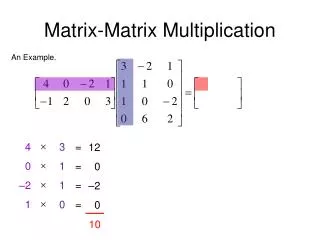
10. Distance Products • The distance product , where A is an matrix, B is , and C is matrix, is defined as follows: • Recall: if W is an n x n matrix of the edge weights of a graph then is the distance matrix of the graph. • Lemma by Alon: can be computed almost as fast as “regular” matrix multiplication:

11. State-of-the-art APSP • Randomized algorithm by Zwick that runs in time • Intuition: • Computation of all short paths is intensive. • BUT: long paths are made up of short paths: once we pay the initial price we can leverage this work to compute longer paths with less effort. • Strategy: Giving up on certainty - with a small number of distance updates we can be almost sure that any long-enough path has at least one representative that is updated.

12. Basic Operations • Truncation • Replace any entry larger than t with • Selection • Extract from D the elements whose row indices are in A, and column indices are in B. • Min-Assignment • Assign to each element the smallest between the two corresponding elements of D and D‘.

13. Pseudo-code • Simply sample nodes and multiply decimated matrices…

14. On matrices and nodes… • Column-decimated matrix Distance between any two nodes D Shortest directed path from any node to any node in B

15. On matrices and nodes…(2) • Row-decimated matrix Distance between any two nodes Shortest directed path from any node in B to any node

16. What do we prove? • Lemma: if there is a shortest path between nodes i and j in G that uses at most edges, then after the -th iteration of the algorithm, with high probability we have • Meaning: at each iteration we update with high probability all the paths in the graph of a certain length. This serves as a basis for the next iteration.

17. Proof Outline • By Induction: • Base case: easy – the input W contains all paths of length • Induction step: • Suppose that the claim holds for and show that it also holds for • Take any two nodes that their shortest distance is at least . The -th iteration matrix product will (almost certainly) plug in their shortest distance at location (i,j) of D.

18. i k j’ j i’ Why? • Set • The path p from i to j is at least 2s/3. • This divides p into three subsections: • Left – at most s/3 • Right – at most s/3 • Middle – exactly s/3

19. The Details • The left and right “thirds” - help attain the induction step. • The path p(i,k) and p(k,j) are short enough – at most 2s/3  good for previous step: • The middle “third” – ensures the fault probability is low enough. • Prob(no k is selected) = • Probability still goes to 0 (as n tends to infinity) after computation of • entries • iterations

20. So… • Assuming all previous steps were good enough: • With high probability each long-enough path has a representative in B • The update of the D using the product plugs in the correct result. • Note that: • Each element is first limited to s*M • This is necessary for the fast-matrix-multiplication algorithm

21. Complexity • Where does the trick hide? • The matrix alphabet increases linearly with iteration number • The product size decreases with iteration number • For each iteration : • Alphabet size: s*M • Product complexity: , where • Total: • Disregarding the log function, and optimizing between fast and naïve matrix products we get:

22. Fast Product versus Naive *assuming small M

23. Complexity Behavior • For a given matrix alphabet M, we find the cross-over point between the matrix algorithms. • For high r (>M-dependent threshold) we use FMM • Complexity dependent on M • For low r (<threshold) we use naïve multiplication • Complexity not dependent on M • Q: How does complexity change over the iteration number?

24. Pre-processing algorithm • Motivation: • We rarely query all node-pairs • Strategy: • Replace the costly matrix product with 2 smaller products: • Generate data structure such that each query costs only

25. Starting with the query… • Pseudo-code: • What is a sufficient trait of D, such that the returned value will be, with high probability • Answer: with high probability, a node k on the path from i to j should have:

26. Preprocessing algorithm

27. New matrix type • Row&Column-decimated matrix Query data structure for any two nodes D Query data-structure for any 2 nodes in B

28. What do we prove? • Lemma 4.1: If or , and there is a shortest path from i to j in G that uses at most edges, then after the -th iteration of the preprocessing algorithm, with high probability we have . • Meaning: D has the necessary trait: for any path p, if we iterate long enough, then with high probability, for at least one node k (in p(i,j)) the entries d(i,k), d(k,j) will contain shortest paths. Hence, “query” will return the correct result.

29. Proof Outline - preprocess • By Induction: • Base case: easy – B=V, and the input W contains all paths of length . • Induction step: • Suppose that the claim holds for and show that it also holds for • Take any two nodes that their shortest distance is at most . The l-th iteration matrix products (2) will (almost certainly) plug in their shortest distance at location (i,j) of D provided that EITHER or .

30. i k j’ j i’ Why? • Set • The path p from i to j is at least 2s/3. • This divides p into three subsections: • Left – at most s/3 • Right – at most s/3 • Middle – exactly s/3

31. The Details • Assume that . • With high probability ( ) there will be k in p(i,j), such that (remember why?) • Both are also in ,since • We therefore attain the induction step: • The path p(i,k) and p(k,j) are short enough – at most 2s/3  good for previous step. • The end-points of these paths (k) are in • Therefore their shortest distance is in D • The second product then updates correctly. (assumption critical here)

32. Where’s the catch? • In APSP, we assure that: • At every iteration l we compute the shortest path of length at most . • BUT: we had to update all pairs each time • In the preprocess algorithm, we assure: • At every iteration l, we compute the shortest path of length at most only for a selected subset. • BUT: this subset covers all possible subsequent queries, with high probability.

33. Complexity • Matrix product: instead of operations we only get • As before, for each iteration , the alphabet size is s*M. • Total complexity: • No matrix-product switch here!

34. Performance • For small M, as long as the number of queries is less than we get better results than APSP. • For small M: • The algorithm overtakes Goldberg’s algorithm, if the graph is dense • For a dense-enough graph , we can run many SSSP queries and still be faster:

35. The larger picture • We saw: • Alg1: heavy pre-processing, light query • Alg2: light pre-processing, heavy query • Alg3: ? Query-oriented (APSP) Preprocess- oriented (pre-process)

36. The Third Way • Suppose we know in advance the we require no more than queries. • We use the following: • Perform iterations of the APSP algorithm • Perform iterations of the pre-process algorithm • Take the matrix B from the last step of step 1. The product returns in any shortest-distance query.

37. Huh? • After the first stage  D holds all the shortest path of all “short” paths, of lengths at most with high probability. • When the second starts stage it can be sure that the induction holds for all • The second stage takes care of the “long” paths, with respect to querying. Meaning: • If the path is long it will have a representative in one of the second-phase iterations • If it is too-short – it will fall under the jurisdiction of the first stage.

38. Complexity • The first stage ( updates) costs at most • The second stage costs only • The query costs • For example – if want to answer a distance query in , we can pre-process in time

39. Q&A (I ask - you answer) • Q: Why couldn’t we sample B in the query step of Alg2 – the one that initially costs O(n)? • A: Because if the path is too short – we will have no guarantee that it will have a representative in B. Alg3 solves this because short distances are computed rigorously. • Conclusion: the less we sample out of V when we query, the more steps we need to run APSP to begin with.

40. Final Procedure • Given q queries, determine the query complexity using . • This assumes M is small enough so that we use fast product. Otherwise compare to • Execute alg3 using steps of APSP and steps of pre-process • Query all q queries.

41. Summary • For the problem we defined: directed graph, with integer weights, whose absolute value is at most M, we have seen: • Alg1: State-of-the-art APSP in • Alg2: State-of-the-art SSSP in • Alg3: A method to calibrate between the two, for a known number of queries.

42. Thank You!