ADPCM Decode
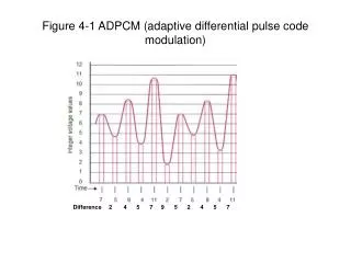
ADPCM Decode. Scott J. Weber Reconfigurable Computing. ADPCM. Adaptive Differential Pulse Code Modulation 4:1 Compression Quantize difference between the speech signal and a prediction that has been made of the speech signal

ADPCM Decode
E N D
Presentation Transcript
ADPCM Decode Scott J. Weber Reconfigurable Computing
ADPCM • Adaptive Differential Pulse Code Modulation • 4:1 Compression • Quantize difference between the speech signal and a prediction that has been made of the speech signal • Decode by adding the quantized difference signal to the predicted signal to reconstruct the speech signal • Adaptive prediction and quantization aid performance • UCLA Mediabench implementation
Spatial ADPCM Decode • Design contains three pieces of computation • Feed back Step Calculator • Feed Forward ShiftAdd Calculator • Approximates vpdiff = (delta * 0.5) * step / 4 • delta is the input sample • Feed back Valpred Calculator
Step Calculator • Low 3 bits of the 4 bit delta (input sample) are used to do a lookup in the IndexTable • Accumulator with clamp at <0 and >88 • Index is used to do a lookup in the stepsizeTable • The result of the stepsizeTable is the STEP fed forward to the ShiftAdd Calculator
ShiftAdd Calculator • STEP was calculated on the previous iteration by the Step Calculator • Approximates vpdiff = (delta * 0.5) * step / 4 • {IN[3], IN[2], IN[1], IN[0]} is delta • vpdiff is the output and is fed forward to the Valpred Calculator
Valpred Calculator • Input is vpdiff as calculated by the ShiftAdd Calculator • Accumulator with 16-bit clamp • Result is the decompressed sample
Feedback Issue • Feed back that exists in the Step and Valpred Calculators is an bottleneck for the spatial design • Smallest cycle constraint achieved was 15 cycles • Results in a 15-Slow design
Spatial Design • Implemented the 15-Slow design • Consumed 315 BLBs, 11 Levels, and had a latency of 106 cycles • Aspect ratio was 5 to 1 • At 4 ns cycles in a 15-Slow design with one stream, the resulting throughput was one sample every 60 ns • Sequential design had an average throughput of 143.5 ns on ribbit • Spatial design is only 2.39x faster than the sequential design • If the cycle constraint could be removed, then the speed improvement would be 35.88x
15-Slow ADPCM Decode • Finding 15 independent stream is difficult • 8-track or 4-track recordings could exploit 15-Slow or 16-Slow • Majority of the data is one input stream • 15-Slow results in 1/15 efficiency for the spatial implementation • Attempted to remove the 15-Slow behaviour
Residual Accumulator Architecture • Possible to remove the cycle constraints if the clamping behaviour were removed (bit pipelining)
Residual Accumulator Architecture • Increases latency of the design, but removes the cycle constraint • Residual is defined as the amount the accumulator is out of a range • By feeding back this residual, the accumulator will, after a given number of cycles, come back into the range • By feeding forward the residual, the result can adjust the accumulator result by adding the calculated residual • When the feed back residual is added into the accumulator, it must also be subtracted from the feed forward residual • Feed back residual allows the accumulator’s 0 base to float • Feed forward residual corrects the accumulator to the reference 0 base
Residual Accumulator Architecture Feed Back Residual Feed Forward Residual Residual Calculator + + - + +
Residual Calculator • Clamp values are floating with the accumulator • Attempted to build with the residual being the difference between two sequential accumulator results and knowledge of which clamp has been exceeded • Example (0 and 88 clamps) • Say 90 is seen, ((88-88)-(90-88)) = -2, residual is -2, (90-2) = 88 • Say 98 is seen, ((90-88)-(98-88)) = -8, residual is -8, (98-10) = 88 • Say 97 is seen, ((98-88)-(97-88)) = 1 , residual is 0, (97-10) = 87 • Since we are over 88, getting a positive difference means we are below 88 • Say 99 is seen, ((97-88)-(99-88)) = -2, residual is -2, (99-12) = 87 • This result is wrong, it should be 88, since the new base is 98 not 99, but that would have required knowledge of the last difference being a 1 • That is a cycle constraint
Residual Calculator • Perhaps there is a way to do this and I have been side stepping it • The discovery of the structure would remove a class of feed back • Seems like the cycle is just being pushed forward • I went ahead and implemented the accumulator design that I described in C, but I let the error remain • I wanted to see how the quality of the results degraded with it • ADPCM is a predictive method, the thought was that perhaps this little error would not explode on me • If the error were acceptable then the cycle constraint could be decreased
Quality vs. Capacity • The Step Calculator and the Valpred Calculator were implemented with Residual Accumulators • The depth of the feedback ranged from 1 to 32 • The results show that the feedback cycle can be closed some, but not completely
Quality vs. Capacity • The average magnitude that the samples are off is under 1000 in a range of 0 to 32767 for depths less than 16 • As the depth increases past 16, the quality quickly decreases. • At depths past 25, the differences seem to become chaotic which may be a result of errors canceling out magnitude differences • A true test would be to actually listen to the decoded signal
Quality vs. Capacity • For throughput rates at 30 ns or greater, the quality of the decoded signal is probably acceptable • At 30 ns, the spatial implementation would have a 5x speedup over the sequential implementation
Architectural Improvement • The feed back that exists in the design results in a 15-slow implementation on the HSRA • A 15-Slow design is only 1/15 efficient in a spatial design • The use of multiple contexts would be an effective way to have a more area efficient design • Multiple contexts would allow the cycle constraint to be potentially decreased since resources are closer in the form of cached hardware
Multiple Contexts • Assume we have a C cycle constraint design with C contexts • We are 1/C efficient in a spatial design • In a multi-contexted design where the C’s match, we are fully efficient in mapped LUT utilization • Only the necessary hardware is resident in each of the C cycles • If there are less contexts than there are constraint cycles then the design would require more LUTs and area • Still more efficient than the spatial design • In a feed back design, multiple contexts allow an area/time tradeoff • The bonus is that the area decreases, but the throughput does not necessarily increase
Multiple Contexts • In ADPCM decode, the Step Calculator is 15-Slow and could be implemented with multiple contexts • The ShiftAdd Calculator is completely feed forward, but is only receiving a new input every 15 cycles, so it too could be designed with multiple contexts to save area and maintain the same relative throughput • The Valpred Calculator is 15-Slow and could be implemented with multiple contexts • With multiple contexts, it is possible to have the same throughput as a completely spatial design with a lower area given that the spatial design has a limiting cycle constraint
SCORE • ADPCM decode can be split into three compute elements • Step Calculator (1 page) (C1-Slow) (feed back) • ShiftAdd Calculator (2 pages) (feed forward) • Valpred Calculator (1 page) (C2-Slow) (feed back) • Only one of the three designs is resident on the HSRA • Produce streams for the next compute element to consume • Productions and consumptions have a static size so a static buffer could be used • Static buffer would be a memory block that is always resident • Area efficient design that does not allow feed forward designs to be starved or feed back designs to be saturated with input streams
SCORE • Allow Step Calculator (C1-Slow) to run for N1 cycles to produce N1/C1 items for the ShiftAdd Calculator • Allow ShiftAdd Calculator to run for N1/C1 cycles to consume the N1/C1 items produced by the Step Calculator and produce N1/C1 items for the Valpred Calculator • Allow Valpred Calculator (C2-Slow) to run N1/C1 * C2 cycles to consume the N1/C1 items produced by the ShiftAdd Calculator and produce N1/C1 outputs • Important that N1is sufficiently large in order to accommodate for the reconfiguration time • Since N1/C1 items are produced and consumed in each design at known rates (Step Calculator (every C1 cycles), ShiftAdd Calculator (every cycle), Valpred Calculator (every C2 cycles)), the productions and consumptions are statically schedulable
SCORE • Possible to have two static buffers and allow two designs to be resident simultaneously • Step Calculator produces to the first static buffer • ShiftAdd Calculator consumes from the first static buffer and produces for the second static buffer • Valpred Calculator consumes from the second static buffer • Step Calculator and Valpred Calculator could be running simultaneously since they have different buffers
POWER • The total energy of the spatial design for decoding a 2.3 million sample adpcm file is 234.298981966 J (Kip’s numbers) • Numbers for the sequential design are not available yet
POWER • Most nodes have an activity rate less than 0.1 • The spatial design’s LUT switching activity factor was 0.043 • Supports the theory that there are highly-correlated (low activity) nodes
Enhancements • RTL type language not structural Java for large designs • Auto-placement support for cascadeLUTs
Summary • Difficult to exploit performance in spatial feed back designs • Temporal pipelining (C-Slow) designs requires independent streams to exist • Multiple contexts allow area to be decreased in feed back designs with little or no cost in performance • Intelligent partitioning into compute pages decreases area with some cost to performance • Residual accumulator could work if quality degradation is acceptable • Curious about the Spatial vs. Temporal energy comparison • Spatial ADPCM decode has several low activity nodes as theorized