Download
1 / 34
340 likes | 501 Views
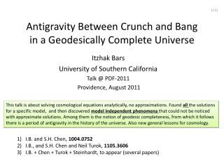
Antigravity Between Crunch and Bang in a Geodesically Complete Universe. Itzhak Bars University of Southern California Talk @ PDF-2011 Providence, August 2011.

E N D
Antigravity Between Crunch and Bang in a Geodesically Complete Universe Itzhak Bars University of Southern California Talk @ PDF-2011 Providence, August 2011 This talk is about solving cosmological equations analytically, no approximations. Found all the solutions for a specific model, and then discovered model independent phenomena that could not be noticed with approximate solutions. Among them is the notion of geodesic completeness, from which it follows there is a period of antigravity in the history of the universe. Also new general lessons for cosmology. • I.B. and S.H. Chen, 1004.0752 • I.B., and S.H. Chen and Neil Turok, 1105.3606 • I.B. + Chen + Turok + Steinhardt, to appear (several papers)
Cosmology with a scalar coupled to gravity Including relativistic matter and curvature 6 parameters 4=b,c,K,ρ0 2=(4-2) initial values Also anisotropic metrics : Kasner, Bianchi IX. Two more fields in metric important only near Big Bang V Analytically solved with this V: found ALL solutions Generic solution is geodesically incomplete in Einstein gravity. There is a subset of geodesically complete solutions only with conditions on initial values and parameters of the model.
For geodesic compleness: a slight extension of Einstein gravity (with gauge degrees of freedom) Local scaling symmetry (Weyl): allows only conformally coupled scalars (generalization possible) (Plus gauge bosons, fermions , more conformal scalars , in complete Weyl invariant theory.) (f,s)(f,s)eλ(x), gmngmne-2λ(x) no ghosts gravitational parameter A prediction of 2T-gravity in 4+2 dims. Also motivated by colliding branes scenario. Fundamental approach: Gauge symmetry in phase space I.B. 0804.1585, I.B.+Chen 0811.2510 Khury + Seiberg +Steinhardt + Turok McFadden + Turok 0409122 Gauge symmetry leftover from general coordinate transformations in extra 1+1 dims. This is not the whole story: Einstein gauge is valid only in a patch of spacetime, Can dynamics push this factor to negative values? ANTIGRAVITY in some regions of spacetime?
Conformal factor of metric =1 for any metric. For all t,x dependence. FRWg Nothing singular in γ-gauge Plus the energy constraint: H=0 This is equivalent to the 00 Einstein eq. G00=T00 which compensates for the ghost. BCRT transform Bars Chen Steinhardt Turok Positive region BB singularity at aE=0 in E-gauge : gauge invariant factor vanishes in γ-gauge, or any gauge!!
Analytic solutions – all of them!! Special case: Completely decoupled equations, except for the zero energy condition. Solutions are Jacobi elliptic functions, with various boundary conditions. BCST transform Friedmann equations become : First integral Particle in a potential problem, intuitively solved by looking at the plot of the potential. Generic solution has
K=0 case quartic potentials E(φ)=E+ρ ≥ E(s) E(s)=E>0 f() , s () = A x F[sn(z|m), cn(z|m), dn(z|m)] z=(τ- τ0)/T A,m,T depend on b,c,K,ρ0,E f(),s () perform independent oscilations For generic initial conditions, the sign of (f2-s2)() changes over time. Generic solution is geodesically incomplete in the Einstein gauge. Geodesically complete with the natural extension in f,sspace. There are special solutions that are geodesically complete in the restricted Einstein frame, but must constrain parameter space.
7/11 Geodesically complete larger space: φγ,sγ plane s Generic solution: f(),s () periodic parametric plot using Mathematica A smooth curve that spans the various quadrants (not shown) Closed curve if periods relatively quantized. Recall Kruskal-Szekeres versus Schwarzchild; now in field space. | φ|<|s| big bangs or big crunches in spacetime at the lightcone inf,s field space. f | φ|>|s| Generic solution is a cyclic universe with antigravity stuck between crunch and bang! Probably true for all V(σ). | φ|>|s| | φ|<|s| No signature change |z| BCST Transform E-gauge to γ-gauge
8/11 Geodesically complete solutions in the Einstein gauge, without antigravity s Conditions on 6 parameter space: (1) Synchronized initial values f(0)=s (0)=0 (2) Relative quantization of periods Pf(5 parameters)=nPs(5 parameters) f b<0 Example n=5 5 nodes in picture f() aE() Cyclic universe s() σ() b>0 Universe expands to infinite size, turnaround at infinite size
9/11 Anisotropy If K≠0, ds3=Bianchi IX (Misner) K0 In Friedmann equations, 2 more fields Friedman Eqs: kinetic terms for α1, α2 just like σ, plus anisotropy potential if K≠0 + p1=(aE)2∂τα1 etc. Free scalars if K=0, then canonical conjugate momenta p1,p2 are constants of motion. Near singularity, kinetic terms dominate, so all potentials, including V(σ) negligible. Then σ momentum q is also conserved near the singularity. For a range of q,p1,p2 mixmaster universe is avoided when σ is present (agree with BKL, etc.) Without potentials can find all solutions analytically for any (initial) anisotropy momenta p1,p2; or σ momentum q including the parameters K,ρ0.
10/11 q= σ momentum, q=(aE)2∂τσ p= anisotropy momentum p1=(aE)2∂τα1 etc. Antigravity Loop (K=0 case) K=0: p1,p2 are conserved throughout motion. q changes during the loop because of V(σ). If small loop, ≈no change. This picture for K=0 ATTRACTOR MECHANISM !! if p1 or p2 is not 0 : both f,s 0 at the big bang or crunch singularity, FOR ALL INITIAL CONDITIONS. φ -s= ALWAYS a period of antigravity sandwiched between crunch and bang φ+s= Duration of loop : (p2+q2)1/2/ρ
11/11 What have we learned? • Found new techniques to solve cosmological equations analytically. • Found all solutions for several special potentials V(σ). • Several model independent general results: geodesic completeness, • and an attractor mechanism to the origin, f,s0, for any initial values. • Antigravity is very hard to avoid. Anisotropy + radiation + KE requires it. • Studied Wheeler-deWitt equation (quantum) for the same system, can solve some cases exactly, others semi-classically. Same conclusions. • Will this new insight survive the effects of a full quantum theory (very likely yes). Should be studied in string theory. • These phenomena are direct predictions of 2T-physics in 4+2 dimensions. • Open: What are the observational effects today of a past antigravity period? This is an important project. Study of small fluctuations and fitting to current observations of the CMB (under investigation).
12/14 Antigravity Loop This picture for K≠0 q,p1,p2 change during each loop (if loop is large) because of the potentials, but trajectory always returns to the origin and connects gravity antigravity regions
K > 0 case K < 0 case E E E . E*=-K2/(16c) E*=K2/(16b) Higher level E>E*, with Es=E, Ef=E+ρ Similar behavior to K=0 case. Lower level E,Ef<E*, with Es=E, Ef=E+ρ s oscillates in the Vs well, while f oscillates outside the Vf hill. Then for any initial values there is a finite bounce at size aE ≠0, no antigravity. Higher level E>0, with Es=E, Ef=E+ρ Similar behavior to K=0 case. Lower level E*<E<0, with Es=E, Ef=E+ρ All solutions are geodesically incomplete in the Einstein gauge. There is no way to avoid antigravity.
14/14 bang turnaround Crunch
Quantization of mini superspace The Wheeler- deWitt Equation Completely separable when When f(s/φ)=0, this is the quantum relativistic harmonic oscillator in 1+1 dimensions Radiation adds just a constant, so it amounts to a new energy level, rather than zero on the right hand side, therefore easily handled. Anisotropy adds a term proportional to WdW eq. is no longer separable, but we can find approximate solution near the singlularity and determine the behavior. -1
Quartic potentials f,s perform independent oscilations. For arbitrary b,c and/or arbitrary initial conditions, the sign of (1-s2/f2) changes over time. E(φ)=E+ρ≥E(s) E(s)=E>0 Geodesically complete (ii)
Still open question If we allow the generic solutions for which (1-s2/φ2) changes sign, what is the observable effect in our patch of the universe? These solutions are not geodesically complete in the Einstein frame, but are non-singular, and geodesically complete in the gamma frame (and also in general frame)
Gravity as background in 2T-physics 0804.1585 [hep-th] Compare to flat case Sp(2,R) algebra puts kinematic constraints on background geometry : homothety Lie derivative Solve kinematics, and impose Q11=Q12=0: Get all shadows, e.g. conformal shadow.
IB: 0804.1585 IB+S.H.Chen 0811.2510 Gravity & SM in 2T-physics Field Theory Gauge symmetry and consistency with Sp(2,R) lead to a unique gravity action in d+2 dims, with no parameters at all. Pure gravity has three fields: GMN(X), metric W(X), dilaton W(X), appears in δ(W) , and more … No scale, a a The equations of motion reproduce the Sp(2,R) constraints, called kinematic equations, (proportional to δ’(W), δ’’(W)), and also the dynamical equations (proportional to δ(W)).
32/26 2T Gravity triplet has unique couplings to matter: scalars, spinors & vectors. Imposes severe constraints on scalar fields coupled to gravity. a a
IB+S.H.Chen 0811.2510 33/20 Solve Sp(2,R) kinematic constraints (homothety) a Conformal scalar, Weyl symmetry
Coupling many scalars. Generating scales. Effects on the gravitational constant and on cosmology. All shadow scalars must be conformal scalars (or similar). NO DIMENSIONFUL CONSTANTS. a . a Can it change sign as a result of dynamics? In the history of the universe? Or in some patches of space-time? If so, are there observational effects in our patch of spacetime? Effect on cosmology ? 34