Mise en situation...
Travaux pratiques de mécanique analytique Simulation en temps réel du mouvement d’un pendule double. X. Y. Mise en situation. Positions:. Point A: (l sin q , -l cos q ). Point B: (l.(sin q + sin f ), -l.(cos q + cos f )). Vitesses:.

Mise en situation...
E N D
Presentation Transcript
Travaux pratiques de mécanique analytiqueSimulation en temps réel du mouvement d’un pendule double
X Y Mise en situation... Positions: Point A: (l sin q, -l cos q) Point B: (l.(sin q + sin f ), -l.(cos q + cos f)) Vitesses: Point A: (l dq/dt cos q, l dq/dt sin q) Point B: (l.(dq/dt cos q + df/dt cos f), l.( dq/dt sin q + df/dt sin f )) m g l = 1 m l2 = 1
Lagrange (1) L = T - V pour toute les masses du système vitesse scalaire de la masse condidérée
V = mgh = - mgl cos q - m g l (cos q + cos f ) L = T - V = + mgl cos q + m g l (cos q + cos f ) Lagrange (2)
ODE45 Fonction de dérivationdécrivant le système différentiel Avant Après Ordre des équations du système 2 ( , ) Fonction différentielle ODE45
ODE45 Fonction de dérivationdécrivant le système différentiel Avant Après Ordre des équations du système 2 ( , ) Définition des vecteurs utilisés
ODE45 Fonction de dérivationdécrivant le système différentiel Avant Après Ordre des équations du système 2 ( , ) Définition des vecteurs utilisés
Fonction de dérivation function [ dy ] = dp ( t, y )
s = sin( - ) c = cos( - ) Variables temporaires function [ dy ] = dp ( t, y )
s = sin( - ) c = cos( - ) Mise en correspondance function [ dy ] = dp ( t, y ) dy(1) = y(2)
s = sin( - ) c = cos( - ) Mise en correspondance function [ dy ] = dp ( t, y ) dy(1) = y(2) dy(3) = y(4)
s = sin( - ) c = cos( - ) Mise en correspondance function [ dy ] = dp ( t, y ) dy(1) = y(2) dy(3) = y(4) dy(2) =
Search and replace function [ dy ] = dp ( t, y ) s = sin( - ) c = cos( - ) dy(1) = y(2) dy(3) = y(4) dy(2) =
Search and replace function [ dy ] = dp ( t, y ) s = sin( - ) c = cos( - ) dy(1) = y(2) dy(3) = y(4) dy(2) =
Search and replace function [ dy ] = dp ( t, y ) s = sin( - ) c = cos( - ) dy(1) = y(2) dy(3) = y(4) dy(2) =
Search and replace function [ dy ] = dp ( t, y ) s = sin( y(1) - ) c = cos(y(1) - ) dy(1) = y(2) dy(3) = y(4) dy(2) =
Search and replace function [ dy ] = dp ( t, y ) s = sin( y(1) - y(3) ) c = cos(y(1) - y(3) ) dy(1) = y(2) dy(3) = y(4) dy(2) =
Search and replace function [ dy ] = dp ( t, y ) s = sin( y(1) - y(3) ) c = cos(y(1) - y(3) ) dy(1) = y(2) dy(3) = y(4) dy(2) =
Search and replace function [ dy ] = dp ( t, y ) s = sin( y(1) - y(3) ) c = cos(y(1) - y(3) ) dy(1) = y(2) dy(3) = y(4) dy(2) =
Search and replace function [ dy ] = dp ( t, y ) s = sin( y(1) - y(3) ) c = cos(y(1) - y(3) ) dy(1) = y(2) dy(3) = y(4) dy(2) =
dy(2) = dy(4) = Search and replace function [ dy ] = dp ( t, y ) s = sin( y(1) - y(3) ) c = cos(y(1) - y(3) ) dy(1) = y(2) dy(3) = y(4)
dy(2) = dy(4) = Fonction différentielle ODE45 function [ dy ] = dp ( t, y ) s = sin( y(1) - y(3) ) c = cos(y(1) - y(3) ) dy(1) = y(2) dy(3) = y(4)
options = odeset('RelTol',1e-8); [t,angle] = ode45('dp',[0:0.1:100],[1 1 10 0],options); Système à résoudre Temps: de 0 à 100 secondes par pas de 0,1 sec Conditions initiales: Résolution numérique
plot ( x , y ) ( 0 , 0 ) ( Ax , Ay ) ( Bx , By ) Variables utilisées
%Allocation mémoire x=zeros(3,1); y=zeros(3,1); %Calcul de coordonnées x(2)=10*sin(angle(1,1)); y(2)=-10*cos(angle(1,1)); x(3)=x(2)+10*sin(angle(1,3)); y(3)=y(2)-10*cos(angle(1,3)); %Préparation session graphique et premier affichage figure; axis([-30 30 -30 30]) hold on; line(x,y,'LineWidth',2); Premier affichage
Boucle d’affichage %Boucle d'affichage for i=1:1000 x(2)=10*sin(angle(i,1)); y(2)=-10*cos(angle(i,1)); x(3)=x(2)+10*sin(angle(i,3)); y(3)=y(2)-10*cos(angle(i,3)); line(x,y,'LineWidth',2); end
Gestion dynamique %Boucle d'affichage for i=1:100 x(2)=10*sin(angle(i,1)); y(2)=-10*cos(angle(i,1)); x(3)=x(2)+10*sin(angle(i,3)); y(3)=y(2)-10*cos(angle(i,3)); clf; axis([-30 30 -30 30]); line(x,y,'LineWidth',2); drawnow;
Temps réel %Boucle d'affichage for i=1:100 tic; x(2)=10*sin(angle(i,1)); y(2)=-10*cos(angle(i,1)); x(3)=x(2)+10*sin(angle(i,3)); y(3)=y(2)-10*cos(angle(i,3)); while toc<0.1; end; clf; axis([-30 30 -30 30]); line(x,y,'LineWidth',2); drawnow; end
Gestion anciennes positions %Allocation mémoire xold=zeros(3,1); yold=zeros(3,1); %Boucle d'affichage for i=1:100 tic; xold(2)=x(2); yold(2)=y(2); xold(3)=x(3); yold(3)=y(3); x(2)=10*sin(angle(i,1)); y(2)=-10*cos(angle(i,1)); x(3)=x(2)+10*sin(angle(i,3)); y(3)=y(2)-10*cos(angle(i,3)); while toc<0.1; end; plot(xold,yold,'w','LineWidth',2); plot(x,y,'LineWidth',2); drawnow; end
Propriété 1 Propriété 2 Propriété ... Propriété n Instruction 1 Instruction 2 Instruction ... Instruction n Approche “orienté-objet” Objet graphique Adresse
Approche “orienté-objet” Objet graphique Adresse XData YData ZData Color Style plot axis
Récupération de l’adresse graph1=plot(x,y,'w*','EraseMode','none'); Objet graphique Adresse = 1.05684523 = graph1 XData YData ZData Color Style Instruction
Données en x graph1=plot(x,y,'w*','EraseMode','none'); Objet graphique Adresse = 1.05684523 = graph1 XData = x YData ZData Color Style Instruction
Données en y graph1=plot(x,y,'w*','EraseMode','none'); Adresse = 1.05684523 = graph1 XData = x YData = y ZData Color Style Instruction
Pas de données en z graph1=plot(x,y,'w*','EraseMode','none'); Objet graphique Adresse = 1.05684523 = graph1 XData = x YData = y ZData Color Style Instruction
Couleur graph1=plot(x,y,'w*','EraseMode','none'); Objet graphique Adresse = 1.05684523 = graph1 XData = x YData = y ZData Color = w Style Instruction
Style graph1=plot(x,y,'w*','EraseMode','none'); Objet graphique Adresse = 1.05684523 = graph1 XData = x YData = y ZData Color = w Style = * Instruction
Variable privée graph1=plot(x,y,'w*','EraseMode','none'); Objet graphique Adresse = 1.05684523 = graph1 XData = x YData = y ZData Color = w Style = * EraseMode = none Instruction
Instruction graphique graph1=plot(x,y,'w*','EraseMode','none'); Objet graphique Adresse = 1.05684523 = graph1 XData = x YData = y ZData Color = w Style = * EraseMode = none Instruction = plot
Accès variables membres set(graph1,'XData',xnew,'YData',ynew,'LineWidth',2); graph1 XData YData
Modification données en x set(graph1,'XData',xnew,'YData',ynew,'LineWidth',2); graph1 XData = xnew YData
Modification données en y set(graph1,'XData',xnew,'YData',ynew,'LineWidth',2); graph1 XData = xnew YData = ynew
LineWidth = 2 Modification paramètres divers set(graph1,'XData',xnew,'YData',ynew,'LineWidth',2); graph1 XData = xnew YData = ynew
%Préparation session graphique et premier affichage p=plot(x,y,'EraseMode','none'); q=plot(xold,yold,'w','EraseMode','none'); %Boucle d'affichage set(q,'XData',xold,'YData',yold,'LineWidth',2); set(p,'XData',x,'YData',y,'LineWidth',2); Pour notre problème
%Préparation session graphique et premier affichage p=plot(x,y,'EraseMode','none'); q=plot(xold,yold,'w','EraseMode','none'); %Boucle d'affichage set(q,'XData',xold,'YData',yold,'LineWidth',2); set(p,'XData',x,'YData',y,'LineWidth',2); Approche “orienté-objet”