Artificial Life Lecture 15

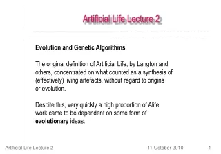
1. Artificial Life Lecture 15 • Some general introduction to ‘Vanilla’ Artificial Neural Networks (ANNs) • Distinctive properties of CTRNNs – Continuous Time Recurrent Neural Networks – as generalised Dynamical Systems • GA+CTRNN exercise, some hints on how to do it …. • … can be followed up in this week’s seminars Artificial Life Lecture 15

2. Many flavours of ANNs Different types of ANNs for different jobs. So far we have looked primarily at ANNs for robot control, e.g. simple feedforward for simple Braitenberg vehicles (for reactive behaviour, in the sense of no internal memory) … and we have mentioned more complex recurrent networks with time involved, such as CTRNNs. But lets start with some of the standard ANNs Artificial Life Lecture 15

3. Pattern recognition A lot – probably by far the most – of ANNs used are not recurrent, are feedforward with no timing issues involved, and can be trained in various possible ways to learn (statistical) input -> output relationships. Let’s recognise that these ANNs probably have near-zero relationship to what actually goes on with real neurons in the brain, and just consider them as potentially really useful pattern-recognisers – all sorts of practical applications. [arguably, to model the temporal aspects of cognition, these ANNs are seriously lacking!] Artificial Life Lecture 15

4. Rapid review Rapid review of the basics of feedforward ANNs BLACK BOX INPUTS OUTPUTS Artificial Life Lecture 15

5. Inputs and Outputs Inputs are a set (or vector) of real numbers (or could be limited to eg just 0s and 1s). Could be data from the stockmarket, past performance of horses in races, pixels from an image etc etc. Artificial Life Lecture 15

6. Inputs and Outputs Outputs: there might be just one, or many outputs of real values (vector). These outputs are, roughly, what a (properly trained) Black Box predicts from the Inputs. E.g. what the Stockmarket index will be tomorrow, how fast the horse will run in the 2:30pm at Newmarket, is the picture like a dog (output 1 high) or a cat (output 2 high) or neither (if both outputs low) Any specific Black Box implements a function from In to Out. Out = BBf(In) Artificial Life Lecture 15

7. Training and Testing If the Black Box is intended to be a dog-recogniser (eg 10x10=100 pixels input, 1 output which should be high for ‘dog’), then ideally it should be testable with all possible input images, and output high only for the doggy ones. There are zillions of possible input images. An ANN is one type of Black Box that can be trained on just a subset, a training set of typical doggy and non-doggy images. Ideally it should then generalise to a test set of images it hasn’t seen before Artificial Life Lecture 15

8. Inside the Black Box Ultimately we will look at multi-layer ANNs, but let’s start simple .. Artificial Life Lecture 15

9. Linear Weighted Sum + Transfer Function The simplest possible ANN with many inputs and one output. TF A 1 ‘neuron’ inside the Black Box, weights on all the 100 inputs I, so the weighted inputs all get summed together at the node. If A is the activation of the node, then Artificial Life Lecture 15

10. Different possible Transfer Functions The output Out is going to be some function of the activation A. Simple possibilities include: Linear Linear + bias NonLinear Step NonLinear Simoid Artificial Life Lecture 15

11. Nonlinear transfer function needed for interesting stuff The first 2 are linear (the second has a bias term b, plus a weight). The next 2 are non-linear, including a sharp step-function or threshold function, and a smoother sigmoid. (Step-function useful if eg Out=1 => dog, Out=0 =>not-dog !!) You can do far more complex pattern-recognition with non-linear functions. The sigmoid is a smooth, and differentiable, version of the step-function, and for practical reasons this turns out useful. So the sigmoid function is one to take note of. Artificial Life Lecture 15

12. Biases The biases just shift the graph left or right. But remember, A was just the weighted sum of inputs Artificial Life Lecture 15

13. Treat bias as another input So if we pretend that there was another input, input value clamped to 1, with a weight of (-b), then we can treat it the same as the other inputs Where w(n+1) = - b And I(n+1) =1 Artificial Life Lecture 15

14. Treating bias as another input Σ TF bias Σ TF bias Artificial Life Lecture 15

15. Treating bias as another input • So when you treat the bias (on any node in the network) as a weight on an input to that node whose input value is clamped to 1 • The equations and the programming come out a lot simpler • And the bias term can be ‘learnt’ by exactly the same method as all the other weights in the ANN are learnt, during training • So from now on we will assume that this trick is being used. Artificial Life Lecture 15

16. The simple Black Box The simplest possible ANN with many inputs and one output. TF Σ Now we have started off looking at this simplest version, a single layer perceptron with 1 output. Could be made a bit more complex if 2 or more outputs (is it a dog? Is it a cat?) Artificial Life Lecture 15

17. Learning Algorithm We still haven’t even started to discuss any training method, whereby the appropriate weights (including biases) can be learnt through exposure to the training set (eg lots of pictures of dogs, cats, other things, with the correct response known for each member of the training set). • Basically there are 2 classes of learning here (ignoring a third of ‘self-organisation’) • Reinforcement Learning • Supervised Learning Artificial Life Lecture 15

18. Jiggling the weights • Basically all these algorithms work on different versions of • Start off with random weights (and biases) in the ANN • Try one or more members of the training set, see how badly the outputs are compared to what they should be (compared to the target outputs) • Jiggle weights a bit, aimed at getting improvement on outputs • Now try with a new lot of the training set, or repeat again, jiggling weights each time • Keep repeating until you get quite accurate outputs Artificial Life Lecture 15

19. Reinforcement In Reinforcement learning, during training an input (‘picture’) is presented to the Black Box, the Output (‘0.75 like a dog’) is compared to the correct output (‘1.0 of a dog’ !!) and the size of the error is used for training (‘wrong by 0.25’) If there are 2 outputs (cats and dogs) then the total error is summed to give a single number (typically sum of squared errors). Eg “your total error on all outputs is 1.76” Note that this just tells you how wrong you were, not in which direction you were wrong. Like ‘Hunt the Thimble’ with clues of ‘warmer’ ‘colder’. Artificial Life Lecture 15

20. Supervised In Supervised Learning the Black Box is given more information. Not just ‘how wrong’ it was, but ‘in what direction it was wrong’ Like ‘Hunt the Thimble’ but where you are told ‘North a bit’ ‘West a bit’. So you get, and use, far more information in Supervised Learning, and this is the normal form of ANN learning algorithm. Artificial Life Lecture 15

21. Reinforcement Learning vs Supervised Genetic Algorithms are a form of Reinforcement learning. So actually a GA is one perfectly good method of ‘evolving’ the weights of an ANN, whether it is 1-layer or multilayer. Encode all the weights (and biases) on the genotype, use a population (randomly initialised), and use errors on the training set as the fitness function. This is just one version of ‘jiggling the weights a bit’ – here it is mutation jiggling the weights. You are, however, usually wasting information that can be used for Supervised Learning. Artificial Life Lecture 15

22. Perceptron Learning Algorithm Gradient descent trying to minimise error. For each training example, input I, expected target output T, actual output O. Error E = T – 0 Jiggle each weight wi by adding a term R x Ii x E, where R is a small constant called the learning rate. This jiggles the weights in the right direction to decrease error, by an amount R which makes it a small jiggle. Gradient descent. Artificial Life Lecture 15

23. The 1-layer algorithm Initialise perceptron with a random set of weights Repeat for each training instance (I,T) do { E = T – Out; for (i=1i<=N;I++) { w[i] = w[i] + R * Ii * E; } } until error acceptably small. Artificial Life Lecture 15

24. What can the simple Perceptron do ? The simplest possible ANN with many inputs and one output. TF Σ We are still looking at this very simple 1-layer perceptron, with 1 (or possibly more) outputs. It can be proved (Perceptron Convergence Theorem) that if there is some set of weights that will do the pattern-recognition, or classification job we want, then the algorithm on previous slide will do the job. Artificial Life Lecture 15

25. However However, it turned out that only relatively simple pattern-recognition, or classification, jobs can be done by the 1-layer perceptron – those that are ‘linearly separable’ This is what Minsky & Papert’s 1969 book was all about – and this shot down ANNs for 2 decades ! Eg the XOR problem cannot be tackled by such a perceptron Artificial Life Lecture 15

26. Linearly separable This is a sketch of how a 2-input, 1-output perceptron needs to classify inputs. It needs to distinguish black dots from open circles, in this training set of 4 examples. In the left case, it can do so with a single straight line – and a 1-layer perceptron can handle this. In the right case, it is not ‘linearly separable’, and cannot manage. Artificial Life Lecture 15

27. Extension to multi-layer perceptrons • It turns out that we can in principle find Black Boxes that do such non-linear separation tasks if • We have an extra ‘hidden’ layer • We have a non-linear transfer function such as the sigmoid at the hidden layer • The tricky bit – we can find a learning algorithm that copes with errors at the different layers, so as to jiggle all the weights appropriately • Backpropagation was the algorithm that broke the logjam Artificial Life Lecture 15

28. Why the sigmoid ? Suppose there was a linear transfer function at the hidden layer Then if you follow all the maths through, it turns out that effectively the hidden layer does not buy you anything extra – it is equivalent to just 1 layer If it has to be non-linear, why not a step function? Turns out that backprop needs a smooth differentiable function, such as this:- Artificial Life Lecture 15

29. How big a hidden layer ? If you just have 1 hidden node, then effectively you are back to a 1-layer ANN You need at least 2, and roughly ‘the more complex the classification task, the more hidden nodes you need’. In principle, absolutely any continuous classification task can be done provided you have enough hidden nodes. But you should not have too many, because of worries about overfitting. Artificial Life Lecture 15

30. Overfitting If you have lots of hidden nodes, then you will have lots of weights (and biases) to learn. Suppose you only have 10 members in your training set, but more than 100 weights, then learning will probably do the equivalent of memorising the idiosyncracies of the input/output pairs – and will not generalise sensibly to new inputs it hasn’t seen before. You can check for overfitting by keeping a few examples back, and after training seeing how well the Black Box generalises to this new test set. Artificial Life Lecture 15

31. Warning on Overfitting – When to worry/not worry If you are training on a subset of all possible example patterns, this is when to worry about overfitting – because overtraining can fixate on the accidental biases of the training set. BUT sometimes you could be training on the WHOLE possible set of examples – then there is no possible overfitting to worry about. Artificial Life Lecture 15

32. So how many hidden nodes, then? Ideally, just enough !! There are (difficult) theoretical answers to this, but one approach is to try different numbers, and see how well the trained ANN generalises to an unseen test set in each case. Pick the best value. In practice, one picks some number by guesswork, experience, asking a friend – and if it works you stick with it, otherwise change! Artificial Life Lecture 15

33. Summary of ‘Vanilla’ feedforward ANNs Feedforward architecture (no time aspects), plastic weights, training ‘trains the weights’ • Weights and biases can be treated the same way • We are going to use errors (output – Target) to jiggle the weights around till error decreases • Reinforcement learning (GAs) is one possibility • Supervised learning uses more information • Present training set, use errors to jiggle weights Artificial Life Lecture 15

34. Typically not feedforward, ‘arrows’ go in all directions! CTRNNs (and other temporal ones) are different DS, Dynamical Systems approach to chosen variables affecting each other in real time Artificial Life Lecture 15

35. CTRNN equations .. ‘fixed weights’ ?!? WIth CTRNNs (continuous-time recurrent NNs), for each node (i = 1 to n) in the network the following equation holds: yi = activation of node i i = time constant, wji = weight on connection from node j to node i (x) = sigmoidal = (1/1+e-x) • i= bias, Ii = possible sensory input. Artificial Life Lecture 15

36. NO !! Best to think of a CTRNN as a CTRDS, where the nodes correspond to any variable that you want to model (incl wts!) Does ‘fixed weights’ mean ‘Cannot Learn’? With CTRNNs, the weights are fixed. The activations in each node change over time, according to the equations (and the time parameters, eg some fast, some slow). With ‘vanilla’ ANNs, the network (after training) has fixed weights. But during training the weights change slowly. Actually, a CTRNN can emulate this sort of weight-changing effect – eg by some of the CTRNN (slow) nodes modelling the (slow) plastic weights Artificial Life Lecture 15

37. ‘Learning’ or ‘Training’ with a CTRNN Because the weights are fixed, you cannot use a weight-changing learning method on a CTRNN. But you can evolve the weights, so that the CTRNN performs the task that you want. You will also be evolving the biases (treat them like other weights) – and you will be evolving the time parameters τi for each node (eg ‘slow’ or ‘fast’). These are all real numbers – code them as doubles or floats Artificial Life Lecture 15

38. Encoding in real values Use doubles or floats on your genotype float my_genotype[LENGTH]; Initialise random population typically to random numbers drawn from an appropriate range. Maybe [-1,+1], or [-2,+2] for a NN, depending on what is reasonable for specific job. Artificial Life Lecture 15

39. Mutating Real numbers Various possibilities for mutating real numbers (see last lecture) Usually a form of 'creep mutation' is used: eg. add a random number in range [-0.1 +0.1] or add a random number drawn from a Gaussian distribution with mean zero, and appropriate range. Rule of thumb is mutate all of them a little bit. Artificial Life Lecture 15

40. More principled way To get a small random change to the vector in N-space that a genotype of N real numbers represents:- • On each of N axes in N-space, construct a vector, length is from a Gaussian mean 0.0 std. dev 1.0 • Add to make a vector in N-space. Normalise length to 1.0. • Multiply by a creep factor, from Gaussian mean 0.0, length ‘creep’ (e.g. 0.1). This is the mutation. Artificial Life Lecture 15

41. Limits for real-valued genes Typically there may be no need to impose lower/upper limits on real-valued genes. But sometimes there is, eg for a time-parameter in a CTRNN it definitely should remain positive. But in this special case it is probably best to have the gene encode a real-value T, and then the actual time parameter is (eg) translated as 10T. Then no absolute need to bound range of T. Artificial Life Lecture 15

42. The GA + CTRNN exercise • One solution is being posted on the website. • Choices to make: genotype will encode parameters of a CTRNN with say NN nodes (NN=2? NN=3?) • How many real numbers? • Weights from each node to all others (jnc self) NN*NN • Each node has a bias, time parameter: 2*NN more • Total: NN*NN + 2*NN real numbers Artificial Life Lecture 15

43. Ranges of numbers Define a range for the weights, biases, eg [-5.0, +5.0] What about the time parameters? These cannot be negative, or indeed zero! So if they are also initialised in the range [-5,5], they must get translated into some positive values. Code on website takes 1.0 + absolute value, i.e. [-5.0, 5.0] -> actual time parameters [1.0, 6.0] Or, you could make actual time parameter = 10T Artificial Life Lecture 15

44. How do you update the nodes? Have an array with current values at each node. Initialise at random. [Or (professional): look into “center-crossing”, Mathayomchan, B. and Beer, RD (2002} ] Update rule, where yi is the current value of ith node Artificial Life Lecture 15

45. Translate update rule Delta_y_i = (Delta_t / tau_i) * RHS of above eqn. It is crucially important to make a sensible choice of your update time-step Delta_t !!! Setting it equal to 1 is almost certainly wrong, and a criminal offence!!! Delta_t should be made significantly smaller than the smallest time parameter in the system. www.informatics.susx.ac.uk/users/inmanh/easy/alife08/TimeSteps.html Artificial Life Lecture 15

46. Why should timesteps be small? www.cogs.susx.ac.uk/users/inmanh/easy/alife09/TimeSteps.html Consider this parabola y = x2 This represents the slope of the tangent. But if you are sliding down the hill, you cannot assume the slope is constant for a distance 1.0, It is only nearly constant for a tiny distance delta_x Artificial Life Lecture 15

47. Timesteps – rule of thumb Take the shortest length of real time within which the system might change more than a minute fraction – e.g. with a CTRNN, the smallest possible time parameter is a guideline, Then, make your update time-step smaller than that, eg 1/10 (or at a pinch, 1/3). Reality check: if making your timestep even smaller will affect the results you get, then it wasn’t small enough! Artificial Life Lecture 15

48. Euler integration So your succession of updates of node values are an approximation (hopefully a close one) to the real-time continuous version. Set up your trial conditions, to see how well the CTRNN performs at this task. In this case: provide a steadily changing input value on one node, and keep track of the output of a designated output-node – how close to right value? Artificial Life Lecture 15