Download
1 / 23
240 likes | 360 Views
Observations of Large Scale Structure: Measures of Galaxy Clustering. Kaz Sliwa Ruben Pinto Marc Cassagnol. The Distance Ladder. There is clearly a hierarchy of structure in the universe: Stars > Star Clusters > Galaxies > Galaxy Clusters > Superclusters

E N D
Observations of Large Scale Structure: Measures of Galaxy Clustering Kaz Sliwa Ruben Pinto Marc Cassagnol
The Distance Ladder • There is clearly a hierarchy of structure in the universe: • Stars > Star Clusters > Galaxies > Galaxy Clusters > Superclusters • Is there any larger structures than this? • Before 1980: Nothing larger. 1980’s: Redshift data revealed more interesting structures. Very non-spherical structures such as …….
Voids • Vast empty spaces between filaments, anywhere from 10 – 150 Mpc in diameter • Few or no galaxies are contained in these regions • Strangely large voids (500+ Mpc) are called supervoids • About 27 known supervoids.
Filaments • Sponge-like, or thread-like structures, which are 70-150 Mpc long • Form boundary between voids • Composed of galaxies, particularly dense regions of a filament are called superclusters.
Surface Brightness Fluctuation (SBF) Method • This technique is used to find distances to galaxies, and can be used where individual stars cannot be resolved. • The brightness of each pixel will fluctuate a certain amount, depending on the distance to the galaxy. • Further away galaxies produce smaller fluctuations. • N = number of stars per pixel of detector.
Measures of Galaxy Clustering • If galaxies were distributed uniformly throughout space with average spatial density n per cubic megaparsec, then the probability dP of finding a galaxy in a volume dV1 would be the same everywhere, dP = ndV1. • If galaxies tend to cluster together then the probability of having a galaxy in another random volume dV2 is greater if the separation r12between the two regions is small. • However, the galaxies are not scattered randomly throughout space and thus the joint probability of finding a galaxy within both volumes dV1and dV2 is written as: • Where is the two-point correlation function.
The two-point correlation function describes whether the galaxies are more concentrated or separated than average. • If ξ(r) > 0 at small r, then the galaxies are clustered, and if ξ(r) < 0 then the galaxies are more dispersed. • Generally the correlation function ξ(r) is computed by estimating the galaxy distance from their redshifts, correcting for distortion introduced by the peculiar velocities. • For small separations of r≤ 50h-1 Mpc, the correlation function takes the form: • where r0 is the correlation length, and γ >0.
In the range 2h-1 ≤ r ≤ 16h-1 Mpc where ξ(r) is well measured the correlation length ro ≈ 6h-1 Mpc and γ ≈ 1.5. • An average over many surveys results in ro ~ 5h-1 Mpc and γ ~ 1.8. • Around r ≥ 30h-1Mpc, ξ(r) starts to oscillate around zero. • While galaxies are not clustered randomly, at larger scales it approaches a random distribution.
Kaz4 • The Fourier transform of ξ(r) is the power spectrum P(k): • The power spectrum indicates the amount of clustering on a given length scale. • An important fact is that the power P(k) ∝ V, that is, it scales with volume and is thus not dimensionless.
“Lumpiness” of Galaxy Distribution • < δ2R> is a dimensionless quantity that measures the lumpiness of the galaxy distribution on this scale. • < δ2R> can be related to k3P(k), the dimensionless quantity that defines the fluctuation in density within a volume: where k ≈ R-1 • Often the clustering is parameterized by σ8 which is defined as the fluctuation on a scale of R = 8h-1 Mpc.
Wedge Diagrams • Resemble two pizza slices joined at the apex and provide 3-d view. • Formed because of system of observation used: Cone. • Counter-clockwise 90 degrees for actual view. • Sides “empty” due to gas and dust obscuring optical view on Milky Way’s plane. • 21cm Line reveals galaxies do exist in the plane.
Redshift Measurements • Recession Speed, or redshift is a measure of fractional change in wavelength • Gives us an approximate distance to galaxies that exhibit radial velocities • Doppler formula for speeds well below speed of light: • Doppler relation and Hubble Law gives recession speed:
The Great Wall • Largest known super-structure in the universe. • Very thin, 500 x 300 x 15 light years in size. • It is a filament of galaxies about 200 million light years away from us. • Could be thicker, the plane of the Milky Way obscures our view of the great wall.
The Great Wall (cont’d) • Popular theories do not account for regular “sheet” patterns, or the enormous size. • Covers more than a quarter of northern hemisphere (redshift survey figure). • Overall Picture: Layers of filaments approx 15 Lyrs thick of high density galaxy distribution – between sheets there is empty space. • Recent studies show, that the initial “facts” of the biggest structures in our universe might be a little exaggerated…
Overestimates • Great Wall has great mass – density is larger than surrounding volumes. • Result: pulls in surrounding galaxies. • Note that the cores of walls have not collapsed yet, hence this is the first time galaxies are “falling” and hence these measurements can be made. • Galaxies in front of wall have higher Vr; behind wall lower Vr. • According to recession speeds, the walls are denser than they really are. • Consequently surrounding regions are not that empty • Truth: walls are only a few times denser than the cosmic mean.
Bias • Not every galaxy can be seen; the types of galaxies observed do depend on the system of observation chosen. • Recession speeds need the galaxies to be of a certain lower limit of luminosity; at cz > 40,000kms-1, only the most luminous systems can be plotted (hence thinning out in diagram). • 21cm line: Optical brightness does not matter – E.g. gas rich dwarf galaxies will dominate over luminous Ellipticals that lack HI gas. • No easy task to map the luminosity-varying Universe!