Download
1 / 27
270 likes | 349 Views
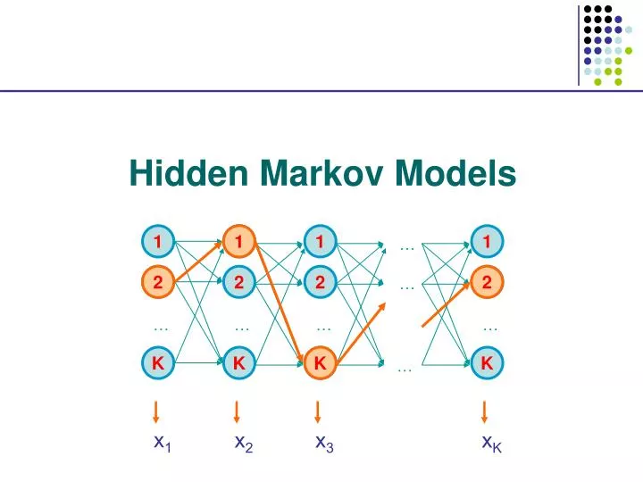
1. 2. 2. 1. 1. 1. 1. …. 2. 2. 2. 2. …. K. …. …. …. …. x 1. K. K. K. K. x 2. x 3. x K. …. Hidden Markov Models. 1. 1. 1. 1. …. 2. 2. 2. 2. …. …. …. …. …. K. K. K. K. …. Generating a sequence by the model.

E N D
1 2 2 1 1 1 1 … 2 2 2 2 … K … … … … x1 K K K K x2 x3 xK … Hidden Markov Models
1 1 1 1 … 2 2 2 2 … … … … … K K K K … Generating a sequence by the model Given a HMM, we can generate a sequence of length n as follows: • Start at state 1 according to prob a01 • Emit letter x1 according to prob e1(x1) • Go to state 2 according to prob a12 • … until emitting xn 1 a02 2 2 0 K e2(x1) x1 x2 x3 xn
Evaluation We will develop algorithms that allow us to compute: P(x) Probability of x given the model P(xi…xj) Probability of a substring of x given the model P(i = k | x) “Posterior” probability that the ith state is k, given x A more refined measure of which states x may be in
The Forward Algorithm fk(i) = P(x1…xi, i = k) (the forward probability) Initialization: f0(0) = 1 fk(0) = 0, for all k > 0 Iteration: fk(i) = ek(xi) l fl(i – 1) alk Termination: P(x) = k fk(N)
Motivation for the Backward Algorithm We want to compute P(i = k | x), the probability distribution on the ith position, given x We start by computing P(i = k, x) = P(x1…xi, i = k, xi+1…xN) = P(x1…xi, i = k) P(xi+1…xN | x1…xi, i = k) = P(x1…xi, i = k) P(xi+1…xN | i = k) Then, P(i = k | x) = P(i = k, x) / P(x) Forward, fk(i) Backward, bk(i)
The Backward Algorithm – derivation Define the backward probability: bk(i) = P(xi+1…xN | i = k) “starting from ith state = k, generate rest of x” = i+1…N P(xi+1,xi+2, …, xN, i+1, …, N | i = k) = li+1…N P(xi+1,xi+2, …, xN, i+1 = l, i+2, …, N | i = k) = l el(xi+1) akli+1…N P(xi+2, …, xN, i+2, …, N | i+1 = l) = l el(xi+1) aklbl(i+1)
The Backward Algorithm We can compute bk(i) for all k, i, using dynamic programming Initialization: bk(N) = 1, for all k Iteration: bk(i) = l el(xi+1) akl bl(i+1) Termination: P(x) = l a0l el(x1) bl(1)
Computational Complexity What is the running time, and space required, for Forward, and Backward? Time: O(K2N) Space: O(KN) Useful implementation technique to avoid underflows Viterbi: sum of logs Forward/Backward: rescaling at each few positions by multiplying by a constant
Posterior Decoding P(i = k | x) = P(i = k , x)/P(x) = P(x1, …, xi, i = k, xi+1, … xn) / P(x) = P(x1, …, xi, i = k) P(xi+1, … xn | i = k) / P(x) = fk(i) bk(i) / P(x) We can now calculate fk(i) bk(i) P(i = k | x) = ––––––– P(x) Then, we can ask What is the most likely state at position i of sequence x: Define ^ by Posterior Decoding: ^i = argmaxkP(i = k | x)
Posterior Decoding • For each state, • Posterior Decoding gives us a curve of likelihood of state for each position • That is sometimes more informative than Viterbi path * • Posterior Decoding may give an invalid sequence of states (of prob 0) • Why?
Posterior Decoding x1 x2 x3 …………………………………………… xN • P(i = k | x) = P( | x) 1(i = k) = {:[i] = k}P( | x) State 1 P(i=l|x) l k 1() = 1, if is true 0, otherwise
Viterbi, Forward, Backward VITERBI Initialization: V0(0) = 1 Vk(0) = 0, for all k > 0 Iteration: Vl(i) = el(xi) maxkVk(i-1) akl Termination: P(x, *) = maxkVk(N) • FORWARD • Initialization: • f0(0) = 1 • fk(0) = 0, for all k > 0 • Iteration: • fl(i) = el(xi) k fk(i-1) akl • Termination: • P(x) = k fk(N) BACKWARD Initialization: bk(N) = 1, for all k Iteration: bl(i) = k el(xi+1) akl bk(i+1) Termination: P(x) = k a0k ek(x1) bk(1)
Higher-order HMMs • How do we model “memory” larger than one time point? • P(i+1 = l | i = k) akl • P(i+1 = l | i = k, i -1 = j) ajkl • … • A second order HMM with K states is equivalent to a first order HMM with K2 states aHHT state HH state HT aHT(prev = H) aHT(prev = T) aHTH state H state T aHTT aTHH aTHT state TH state TT aTH(prev = H) aTH(prev = T) aTTH
Similar Algorithms to 1st Order • P(i+1 = l | i = k, i -1 = j) • Vlk(i) = maxj{ Vkj(i – 1) + … } • Time? Space?
Modeling the Duration of States 1-p Length distribution of region X: E[lX] = 1/(1-p) • Geometric distribution, with mean 1/(1-p) This is a significant disadvantage of HMMs Several solutions exist for modeling different length distributions X Y p q 1-q
Solution 1: Chain several states p 1-p X Y X X q 1-q Disadvantage: Still very inflexible lX = C + geometric with mean 1/(1-p)
Solution 2: Negative binomial distribution Duration in X: m turns, where • During first m – 1 turns, exactly n – 1 arrows to next state are followed • During mth turn, an arrow to next state is followed m – 1 m – 1 P(lX = m) = n – 1 (1 – p)n-1+1p(m-1)-(n-1) = n – 1 (1 – p)npm-n p p p 1 – p 1 – p 1 – p Y X(n) X(1) X(2) ……
Example: genes in prokaryotes • EasyGene: Prokaryotic gene-finder Larsen TS, Krogh A • Negative binomial with n = 3
Solution 3: Duration modeling Upon entering a state: • Choose duration d, according to probability distribution • Generate d letters according to emission probs • Take a transition to next state according to transition probs Disadvantage: Increase in complexity of Viterbi: Time: O(D) Space: O(1) where D = maximum duration of state F d<Df xi…xi+d-1 Pf Warning, Rabiner’s tutorial claims O(D2) & O(D) increases
Viterbi with duration modeling emissions emissions Recall original iteration: Vl(i) = maxk Vk(i – 1) akl el(xi) New iteration: Vl(i) = maxk maxd=1…DlVk(i – d) Pl(d) akl j=i-d+1…iel(xj) F L d<Df d<Dl Pl Pf transitions xi…xi + d – 1 xj…xj + d – 1 Precompute cumulative values
A state model for alignment M (+1,+1) Alignments correspond 1-to-1 with sequences of states M, I, J I (+1, 0) J (0, +1) -AGGCTATCACCTGACCTCCAGGCCGA--TGCCC--- TAG-CTATCAC--GACCGC-GGTCGATTTGCCCGACC IMMJMMMMMMMJJMMMMMMJMMMMMMMIIMMMMMIII
Let’s score the transitions s(xi, yj) M (+1,+1) Alignments correspond 1-to-1 with sequences of states M, I, J s(xi, yj) s(xi, yj) -d -d I (+1, 0) J (0, +1) -e -e -AGGCTATCACCTGACCTCCAGGCCGA--TGCCC--- TAG-CTATCAC--GACCGC-GGTCGATTTGCCCGACC IMMJMMMMMMMJJMMMMMMJMMMMMMMIIMMMMMIII
Alignment with affine gaps – state version Dynamic Programming: M(i, j): Optimal alignment of x1…xi to y1…yjending in M I(i, j): Optimal alignment of x1…xi to y1…yj ending in I J(i, j): Optimal alignment of x1…xi to y1…yjending in J The score is additive, therefore we can apply DP recurrence formulas
Alignment with affine gaps – state version Initialization: M(0,0) = 0; M(i, 0) = M(0, j) = -, for i, j > 0 I(i,0) = d + ie; J(0, j) = d + je Iteration: M(i – 1, j – 1) M(i, j) = s(xi, yj) + max I(i – 1, j – 1) J(i – 1, j – 1) e + I(i – 1, j) I(i, j) = max d + M(i – 1, j) e + J(i, j – 1) J(i, j) = max d + M(i, j – 1) Termination: Optimal alignment given by max { M(m, n), I(m, n), J(m, n) }