Solution Techniques

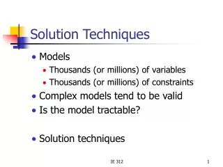
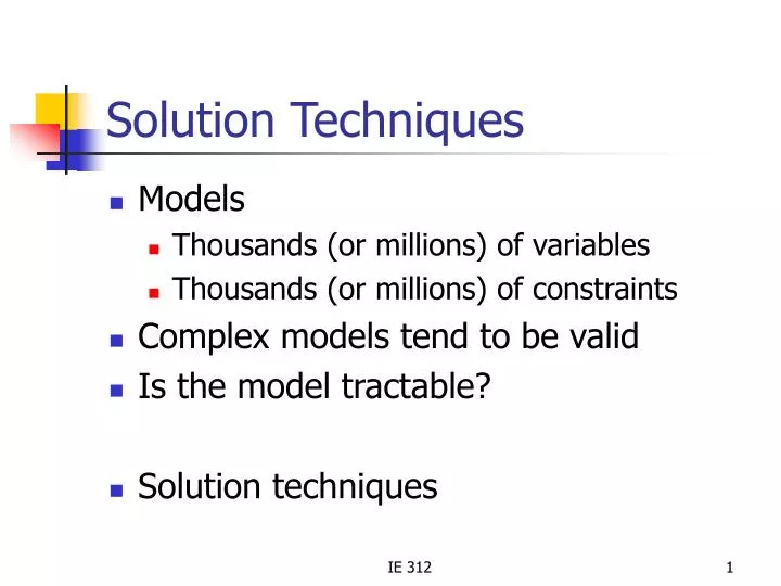
1. Solution Techniques • Models • Thousands (or millions) of variables • Thousands (or millions) of constraints • Complex models tend to be valid • Is the model tractable? • Solution techniques IE 312

2. Definitions • Solution: a set of values for all variables • n decision variables: solution n-vector • Scalar is a single real number • Vector is an array of scalar components IE 312

3. Some Vector Operations • Length (norm) of a vector x • Sum of vectors • Dot product of vectors n = 2 x x j + = j 1 x y 1 1 M + = x y + x y n n n = x y x y j j = j 1 IE 312

4. Neighborhood/Local Search • Find an initial solution • Loop: • Look at “neighbors” of current solution • Select one of those neighbors • Decide if to move to selected solution • Check stopping criterion IE 312

5. Example: DClub Location • Location of a discount department store • Three population centers • Center 1 has 60,000 people • Center 2 has 20,000 people • Center 3 has 30,000 people • Maximize business • Decision variables: coordinates of location IE 312

6. Constraints Must avoid congested centers (within 1/2 mile): IE 312

7. Objective Function 60 = max p ( x , x ) 1 2 + + + - 2 2 1 ( x 1 ) ( x 3 ) 1 2 20 + + - + - 2 2 1 ( x 1 ) ( x 3 ) 1 2 30 + + + + 2 2 1 ( x ) ( x 3 ) 1 2 IE 312

8. Objective Function IE 312

9. Searching IE 312

10. Improving Search • Begin at feasible solution • Advance along a search path • Ever-improving objective function value • Neighborhood: points within small positive distance of current solution • Stopping criterion: no improvement IE 312

11. Local Optima • Improving search finds a local optimum • May not be a global optimum (heuristic solution) • Tractability: for some models there is only one local optimum (which hence is global) IE 312

12. Selecting Next Solution • Direction-step approach • Improving direction: objective function better for than for all value of l that are sufficiently small • Feasible direction: not violate constraints + = + l ( t 1 ) ( t ) x x x Step size Search direction + l ( t ) x x IE 312

13. Step Size • How far do we move along the selected direction? • Usually: • Maintain feasibility • Improve objective function value • Sometimes: • Search for optimal value IE 312

14. Detailed Algorithm 0 Initialize: choose initial solution x(0); t=0 1 If no improving direction x, stop. 2 Find improving feasible direction x (t+1) 3 Choose largest step size lt+1 that remains feasible and improves performance 4 Update Let t=t+1 and return to Step 1 + + = + l ( t 1 ) ( t ) ( t 1 ) x x x + t 1 IE 312

15. Stopping • Search terminates at local optimum • If improving direction exists cannot be a local optimum • If no improving direction then local optimum • Potential problem with unboundedness • Can improve performance forever • Search does not terminate IE 312

16. Local Optimum IE 312

17. Improving Search • Still a bit abstract • ‘Find improving feasible direction’ • How? IE 312

18. Smooth Functions • Assume objective function is smooth • What does this mean? • You can find the derivative Smooth Not Smooth IE 312

19. Gradients • Function • The gradient is found from the partial derivatives • Note that the gradient is a vector = f ( x ) ( f / x , f / x ,..., f / x ) 1 2 n IE 312

20. Example IE 312

21. Partial Derivatives ( ) + + + - 2 2 60 1 ( x 1 ) ( x 3 ) × 1 2 p ( x , x ) x = + 1 2 1 ... [ ] 2 x + + + - 2 2 1 ( x 1 ) ( x 3 ) 1 1 2 × + 120 ( x 1 ) = + 1 ... [ ] 2 + + + - 2 2 1 ( x 1 ) ( x 3 ) 1 2 IE 312

22. Plotting Gradients IE 312

23. Direction of Gradients • Gradients are • perpendicular to contours of objective function • direction most rapid objective value increase • Using gradients as direction gives us the steepest descent/ascent (greedy) IE 312

24. Effect of Moving • When moving in direction x: • The objective function is increased if (Improving direction for maximization) • The objective function is decreased if  > f ( x ) x 0  < f ( x ) x 0 IE 312

25. Feasible Direction • Make sure the direction is feasible • Only have to worry about active constraints (tight/binding constraints) No active constrains <= x 9 One active constraint 1 Active if equality sign holds! IE 312

26. Linear Constraints • Direction Dx is feasible if and only if (iff) IE 312

27. Comments • The gradient gives us • A greedy improving direction • Building block for other improving directions (later) • Conditions • Check if direction is improving (gradient) • Check if direction is feasible (linear) IE 312

28. Validity versus Tractability • Which models are tractable for improving search? • Stops when it encounters a local optimum • This is guaranteed to be a global optimum only if it is unique IE 312

29. Unimodal Functions • Unimodal functions: • Straight line from a point to a better point is always an improving direction IE 312

30. Typical Unimodal Function IE 312

31. Linear Objective • Linear objective functions • Unimodal for both maximization and minimization n  = = f ( x ) c x c x j j = j 1 IE 312

32. Check First calculate Then apply our test to IE 312

33. Optimality • Assume our objective function is unimodal • Then every unconstrained local optimum is an unconstrained global optimum • Note that none of the constraints can be active (tight) IE 312

34. Convexity • Now lets turn to the feasible region • A feasible region is convex if any line segment between two points in the region is contained in the region IE 312

35. Line Segments • Representing a line • To prove convexity, we have to show that for any points in the region, all points that can be represented as above are also in the region ( ) + l - l ( 1 ) ( 2 ) ( 1 ) x x x , [ 0 , 1 ] IE 312

36. Linear Constraints • If all constraints are linear then the feasible region is convex • Suppose we have two feasible points: • How about a point on the line between: IE 312

37. Verify Constraints Hold IE 312

38. Example IE 312

39. Tractability • (This is the reason we are defining all these term!) • The most tractable models for improving search are models with • unimodal objective function • convex feasible region • Here every local optimum is global IE 312

40. Improving Search Algorithm 0 Initialize: choose initial solutionx(0); t=0 1 If no improving direction Dx, stop. 2 Find improving feasible direction Dx (t+1) 3 Choose largest step size lt+1 that remains feasible and improves performance 4 Update Let t=t+1 and return to Step 1 IE 312

41. Initial Feasible Solutions • Not always trivial to find an initial solution • Thousands of constraints and variables • Initial analysis: • Does a feasible solution exist? • If yes, find a feasible solution • Two methods • Two-phase method • Big-M method IE 312

42. Two-Phase Method • Choose a solution to model and construct a new model by adding artificial variables for each violated constraint • Assign values to artificial variables. • Perform improving search to minimize sum of artificial variables • If terminate at zero then feasible model and continue, otherwise stop • Delete artificial components to get feasible solution • Start an improving search Phase I Phase II IE 312

43. Crude Oil Refinery IE 312

44. Artificial Variables • Select a convenient solution • Add artificial variables for violated constraints IE 312

45. Phase I Model s.t. IE 312

46. Phase I Initial Solutions • As before • To assure feasibility • Thus, the initial solution is IE 312

47. Phase I Outcomes • We cannot get negative numbers and problem cannot be unbounded • Three possibilities • Terminate with f =0 • Start Phase II with final solution as initial solution • Terminate at global optimum with f > 0 • Problem is infeasible • Terminate at local optimum with f > 0 • Cannot say anything IE 312

48. Big-M Method • Artificial variables as before • Objective function • Combines Phase I and Phase II search IE 312

49. Terminating Big-M • If terminates at local optimum with all artificial variables = 0, then also local optimum for original problem • If M is ‘big enough’ at terminates at global optimum with some artificial variables >0, then original problem infeasible • Cannot say anything in between IE 312

50. Linear Programming • We know what leads to high tractability: • Unimodal objective function • Convex feasible region • We know how to guarantee this • Linear objective function • Linear constraints • When are linear programs valid? Much stronger! IE 312