Download
1 / 17
200 likes | 467 Views
Radiation Transport. STScI-PRC1996-13a. Current astrophysical research using radiation transport. Interstellar medium: PN evolution Photoevaporation of cometary knots Evolution of proplyds HII formation and evolution Intergalactic medium Photoevaporation of cosmological mini-haloes

E N D
STScI-PRC1996-13a Current astrophysical research using radiation transport • Interstellar medium: • PN evolution • Photoevaporation of cometary knots • Evolution of proplyds • HII formation and evolution • Intergalactic medium • Photoevaporation of cosmological mini-haloes • Cosmological reionization NOAO/AURA (Abell 39) Nakamoto 2001 STScI-PRC1995-45a STScI-PRC1994-24b
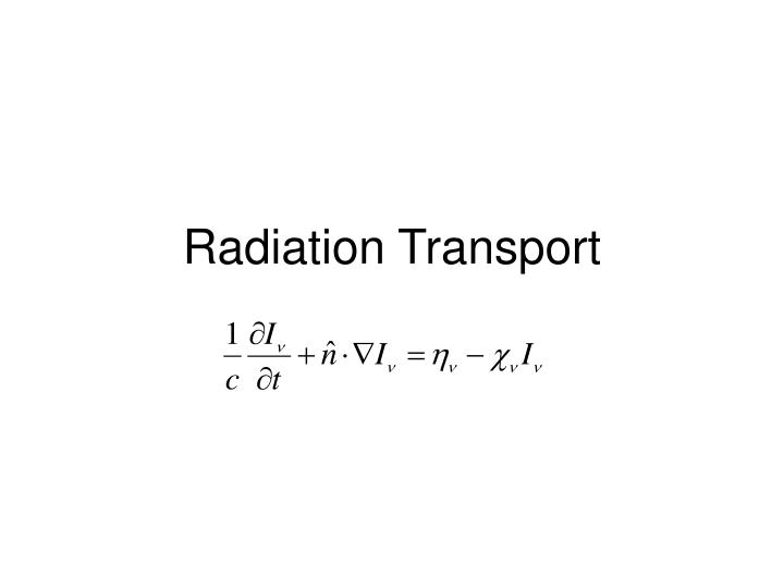
Where is the volume emissivity and is the absorption coefficient. In the absence of emitters or absorbers, the radiation equation becomes: Radiation transport equation: The specific intensity is the energy flux per unit frequency per unit solid angle. The transport equation is then expressed in terms of the specific intensity: The specific intensity is constant along a given ray or characteristic More generally though, along a given characteristic we have: Where we have used the quasi-static approximation and
Source function • If the source function is known then the transport equation can be solved: • Typically the source function (and the optical depth) depend on the chemistry of the material (temperature, degree of ionization) as well as the distribution of the material (density). And the chemistry is usually dependent on the radiation field. However in thermal absorption and emission, the source function is just the Planck function. • More typically in astrophysical plasmas, we have something closer to pure isotropic scattering in which the source function is just the angle averaged specific intensity. • But now the transport equation becomes an integro-differential equation:
Specific intensity Difficulties with calculating specific intensity • Specific intensity is a function of position, time, and direction as well as frequency • Generally has a non-local nature (hard to calculate in parallel) • Feedback between radiation field and material Simplifying factors • Specific intensity often dominated by point sources in which the specific intensity is mono-directional. • Often only need to calculate the specific intensity at a few frequencies around ionization potentials of HI, HeI… • Diffuse field tends to be nearly isotropic • Radiation field quickly adjusts to changes in source terms – quasi-static approximation
Computational Methods • Lambda iteration • Frequency decomposition • Moment methods • Short Characteristics • Hybrid Characteristics • Multiple Wave Fronts
Λ Iteration • Integro-differential equation can be solved by first calculating using the previous value of and then using this to calculate the new value of and then repeating this process until convergence. • Typically, scattering will be isotropic, but rarely will it be coherent. • In HII regions, absorptions are always from the ground state, but recombinations can occur to any excited state followed by a radiative cascade back to the ground state. As a result, the source function for each frequency will depend not only on the mean intensity at that frequency, but on the mean intensity over a wide range of frequencies.
Local averaging of narrow frequency bands • In most astrophysical plasmas we are only interested in modeling the interaction of the radiation field with hydrogen and helium. As a result we are only interested in calculating the specific intensity at frequencies capable of ionizing HI, HeI, and HeII. • Typically the incident radiation field can be integrated over the cross sections so that the optical depth and radiation field at the ionization potentials of HI, HeI, and HeII enables accurate calculations of ionization rates. • Typically the scattered field will contain contributions capable of further ionization from the recombinations of HI, HeI, and HeII. As the temperatures in diffuse astrophysical plasmas are often ~2eV, the scattered photons from recombination will typically have energies within a few eV of the ionization potentials – so the scattered field will contain rather narrow bands. • Three other bound-bound transitions of He are capable of further ionization, but these are also confined to a narrow frequency band with a small doppler width.
Moment methods • For fields that are fairly isotropic (diffuse fields), the specific intensity can be approximated by its various moments.
Then taking the first two moments of the transfer equation in the quasi-static approximation we arrive at: • But now we need some way to close the moment equations. • Eddington factor closure: • Diffusion approximation: where is given by:
Point Sources • Due to the linear nature of the specific intensity, the contribution from point sources can be separated from that due to diffuse scattering. • The diffuse field is often fairly isotropic and can be modeled using some form of moment method. • Solving for the direct field from the point source(s) then reduces to solving the transport equation with no source terms, which reduces to calculating the optical depth from the point source(s) to any given cell. This can be done by some form of ray tracing – short or long characteristics.
Short vs. Long Characteristics • When dealing with point sources, we need to calculate the optical depth to every cell. Since characteristics from the point source to any given cell cross many other cells, we would normally have to add the contributions from cells close to the point source many times. This can be avoided by using short characteristics. And then working our way outwards by interpolating the optical depth at the upwind corners and then adding the local contribution. However, this method is not suited for parallel computations and the interpolation introduces additional numerical diffusion. Rijkhorst (2006)
Hybrid Characteristics Rijkhorst (2006) Hybrid characteristic methods use “short” long characteristics to calculate the optical depth to each cell within each patch combined with “long” short characteristics to accumulate the total optical depth from a given point source.
Non-isotropic fields • In the case of multiple point sources or non-isotropic scattering, neither moment methods nor characteristic methods are well suited. • However, recent advances in computational capability have made five dimensional calculations possible. These calculations basically involve using short characteristics beginning at the outer boundary and interpolating across the grid, however here the calculations can be done in parallel as there are many different directions and the calculations can be done independently. Multiple Wave Front method. Nakomoto (2001)
Comparison project Iliev (2006)
References • Nakamoto T., Umemura M., Susa H., 2001, MNRAS, 321, 593 • Stone J., Mihalas D., Norman M., 1992, ApJS, 80, 819S • Hayes J., Norman M., 2003, ApJS, 147, 197H • Juvela M., Padoan P., 2005, ApJ, 618, 744J • Rijkhorst E., Plewa T., Dubey A., Mellema G., 2006, A&A, 452, 907R • Henney W., 2006, astro-ph, 2626H • Iliev I. et al, 2006, MNRAS, 371, 1057I