Faster Primal-Dual Algorithms for the Economic Lot-Sizing Problem
380 likes | 532 Views
This paper presents advancements in the Economic Lot-Sizing Problem through faster primal-dual algorithms. It reviews previous research and introduces a modified "wave" algorithm that optimally addresses the non-speculative case. The authors evaluate the performance of the new algorithm and provide theoretical insights into its efficiency, achieving O(n) complexity for certain cases. Furthermore, connections to basic algorithm problems and applicability to other inventory issues are discussed. This work enhances understanding of inventory management and computational efficiency in production planning.

Faster Primal-Dual Algorithms for the Economic Lot-Sizing Problem
E N D
Presentation Transcript
Acknowledgment: Thomas Magnanti, Retsef Levi Faster Primal-Dual Algorithms for theEconomic Lot-Sizing Problem Mihai PătraşcuAT&T Research Dan StratilaRUTCOR and Rutgers Business SchoolRutgers University ISMP XX 25 August 2009 TexPoint fonts used in EMF. Read the TexPoint manual before you delete this box.: AAAAAAAAAAAAAA
Outline • Models: • The economic lot-sizing problem. • An important special case: the non-speculative condition. • Overview of previous results. • Review of “wave” primal-dual algorithm of Levi et al (2006). • Main result: a faster algorithm for the lot-sizing problem. • Conclusions: • Connection with basic algorithms problems. O(n)? • Wave primal-dual applicable to other inventory problems. ISMP XX
The Economic Lot-Sizing Problem ISMP XX
An Important Special Case ISMP XX
An Important Special Case ISMP XX
Outline • Models: • The economic lot-sizing problem. • An important special case: the non-speculative condition. • Overview of previous results. • Review of “wave” primal-dual algorithm of Levi et al (2006). • Main result: a faster algorithm for the lot-sizing problem. • Conclusions: • Connection with basic algorithms problems. O(n)? • Wave primal-dual applicable to other inventory problems. ISMP XX
Previous Results on Lot-Sizing Early research: • Introduced by Manne (’58), Wagner and Whitin (’58). • Wagner and Whitin (’58) provide O(n2) for non-speculative case. • Zabel (’64), Eppen et al (’69) obtain O(n2) for general case. • Results on heuristics, to be more efficient than O(n2) in ’70s-’80s. The O(n logn) algorithms: • Federgruen and Tzur (’91), forward algorithm. • Wagelmans et al (’92), backward algorithm, also relate to dual. • Aggarwal and Park (’93), using Monge arrays, generalizations. • These 3 algorithms run in O(n) for non-speculative case. Non-algorithmic results: • Krarup and Bilde (’77) show that above formulation is integral. • Polyhedral results for harder versions, e.g. multi-item lot-sizing: Production Planning by Mixed Integer Programming, Pochet and Wolsey (’06). ISMP XX
Primal-Dual Algorithms for Lot-Sizing Levi et al (’06) : • Obtain primal-dual algorithm for lot-sizing problem. • Proves above formulation is integral as a consequence. • Primal-dual 2-approxim. algorithms for joint replenishment problem (JRP), and for multistage assembly problem. • Algorithms clearly polynomial, authors do not estimate running times. Related primal-dual algorithms for facility location: • Primal-dual algorithms of Levi et al for inventory is rooted in primal-dual approximation algorithm for facility location of Jain and Vazirani (’01). • Thorup (’03) obtains 1.62 algorithm approximation algorithm for facility location with running time Õ(m+n) based on Jain and Vazirani (’01) and Jain et al (’03). Differences: • Algorithms for facility location and lot-sizing are different. • Input size is different: lot-sizing represented as facility would have O(n2) edges. ISMP XX
Outline • Models: • The economic lot-sizing problem. • An important special case: the non-speculative condition. • Overview of previous results. • Review of “wave” primal-dual algorithm of Levi et al (2006). • Main result: a faster algorithm for the lot-sizing problem. • Conclusions: • Connection with basic algorithms problems. O(n)? • Wave primal-dual applicable to other inventory problems. ISMP XX
Wave Primal-Dual Algorithm for Lot-Sizing (Modified, Levi et al ’06) ISMP XX
General • Start with (v,w)=0 and (x,y)=0 • Iteratively increase dual solution, increasing dual objective • At the same time, construct primal solution • When dual objective cannot be increased, primal is feasible • Post-processing step, O(n) • More details • To increase dual objective, we increase budgets vt • At some point, some of the constraints become tight • To keep increasing vt we begin increasing wst for those constraints • At some point some of the constraints become tight • Open s in the primal • Freeze all corresponding vt • Demands t with wst>0 assigned to order s • Remaining free choice—order in which vt are increased ISMP XX
The Wave • start increasing v4 • start increasing w44 • start increasing v3 • order 4 opens, budget 4 freezes demand 4 assigned to order 4 • start increasing w33 • start increasing v2 • start increasing w22 and w32 • order 2 opens, budgets 2 & 3 freeze demands 2 & 3 assigned to order 2 • start increasing v1 • start increasing w11 • order 1 opens, budgets 1 freezes, demand 1 assigned to order 1 • Types of events: • Demand point becomes active • Budget begins contributing to Kt • Order point becomes tight & assoc. ISMP XX
Wave Time and Position Wave time¿ Wave position W ISMP XX
Events: • Demand point becomes active • Budget begins contributing to Kt • Order point becomes tight & assoc. • Algorithms for digital computers: • Goal at end of execution to obtain • primal y and dual v. • Execute (3) from event to event, • instead of continuously • Step (3): • Compute wave position W* when • next order point becomes tight. • Update W:=W*, then updatevandw. ISMP XX
One iteration of (3): • For each unfrozen order point t, • compute position Wtwhen it becomes tight, • assuming no other unfrozen order points • become tight in the meantime. ISMP XX
One iteration of (3): • For each unfrozen order point t, • compute position Wtwhen it becomes tight, • assuming no other unfrozen order points • become tight in the meantime. • Compute W3 ISMP XX
One iteration of (3): • For each unfrozen order point t, • compute position Wtwhen it becomes tight, • assuming no other unfrozen order points • become tight in the meantime. • Compute W3 • Compute W2 ISMP XX
One iteration of (3): • For each unfrozen order point t, • compute position Wtwhen it becomes tight, • assuming no other unfrozen order points • become tight in the meantime. • Compute W3 • Compute W2 • Compute W1 ISMP XX
One iteration of (3): • For each unfrozen order point t, • compute position Wtwhen it becomes tight, • assuming no other unfrozen order points • become tight in the meantime. • Set W' = min{ Wt : t is unfrozen } Lemma:W' = W*, the position when the next order point becomes tight. Wtthat yields the minimum corresponds to the next order point that becomes tight. • Running time O(n3): • One computation of Wttakes O(n). • O(n) computations before an order point • becomes tight. • At most O(n) order points become tight. ISMP XX
One iteration of (3): • For each unfrozen order point t, • compute position Wtwhen it becomes tight, • assuming no other unfrozen order points • become tight in the meantime. • Set W' = min{ Wt : t is unfrozen } Lemma:W' = W*, the position when the next order point becomes tight. Wtthat yields the minimum corresponds to the next order point that becomes tight. • Running time O(n2): • With preprocessing Wttakes O(1) amortized. • O(n) computations before an order point • becomes tight. • At most O(n) order points become tight. ISMP XX
Outline • Models: • The economic lot-sizing problem. • An important special case: the non-speculative condition. • Overview of previous results. • Review of “wave” primal-dual algorithm of Levi et al (2006). • Main result: a faster algorithm for the lot-sizing problem. • Conclusions: • Connection with basic algorithms problems. O(n)? • Wave primal-dual applicable to other inventory problems. ISMP XX
Events: • Demand point becomes active • Budget begins contributing to Kt • Order point becomes tight & assoc • Algorithms for digital computers: • Goal at end of execution to obtain • primal y and dual v. • We will have “tentative” executions • of (3), which may be incorrect. • When we realize an execution is • incorrect, we go back and delete it. • Algorithm terminates => remaining • executions guaranteed correct. ISMP XX
Additional data structure: • Stack D = (ok, ok-1, …, o1) of • provisionally tight order points. • Stack initially empty, at end of loop (2) • will contain the correct order points. • Algorithm: • Start with D=(), t=n. • While t≥1: • 2.1) Compute time when order point tbecomes tight, taking into accountperiods t, …, n but ignoring periods 1, …, t-1. • 2.2) If t becomes tight before ok, delete ok from stack D, and go to 2.1. • 2.3) Add t to stack D, set t:=t-1. ISMP XX
t=3 • Additional data structure: • Stack D = (ok, ok-1, …, o1) of • provisionally tight order points. • Stack initially empty, at end of loop (2) • will contain the correct order points. • Algorithm: • Start with D=(), t=n. • While t≥1: • 2.1) Compute time when order point tbecomes tight, taking into accountperiods t, …, n but ignoring periods 1, …, t-1. • 2.2) If t becomes tight before ok, delete ok from stack D, and go to 2.1. • 2.3) Add t to stack D, set t:=t-1. ISMP XX
s2 e2 s3=e3 • Stack data structure: • Stack D = (ok, ok-1, …, o1) of • provisionally tight order points. • Stack initially empty, at end of loop (2) • will contain the correct order points. • Add information to stack: • E = ((ok, sk, ek), (ok-1, sk-1, ek-1), (o1,s1,e1) of • provisionally tight order points. • sk, …, ek are the demand points that were frozen when ok become tight. • Algorithm: • Start with D=(), t=n. • While t≥1: • 2.1) Compute time when order point tbecomes tight, taking into accountperiods t, …, n but ignoring periods 1, …, t-1. • 2.2) If t becomes tight before ok, delete ok from stack D, and go to 2.1. • 2.3) Add t to stack D, set t:=t-1. ISMP XX
s2 e2 s3=e3 • Stack data structure: • Stack D = (ok, ok-1, …, o1) of • provisionally tight order points. • Stack initially empty, at end of loop (2) • will contain the correct order points. • Add information to stack: • E = ((ok, sk, ek), (ok-1, sk-1, ek-1), …, (o1, s1, e1)) of provisionally tight order points. • sk, …, ek are the demand points that were frozen when ok became tight. • Algorithm: • Start with D=(), t=n. • While t≥1: • 2.1) Compute time when order point tbecomes tight, taking into accountperiods t, …, n but ignoring periods 1, …, t-1. • 2.2) If t becomes tight before ok, delete ok from stack D, and go to 2.1. • 2.3) Add t to stack D, set t:=t-1. • Add further information to stack: • E = ((ok, sk, ek, wk), (ok-1, sk-1, ek-1, wk), …, (o1,s1,e1,w1)) of provisionally tight order points. • wkis the wave position when ok became tight. ISMP XX
w4 • Stack data structure: • Stack D = (ok, ok-1, …, o1) of • provisionally tight order points. • Stack initially empty, at end of loop (2) • will contain the correct order points. • Add information to stack: • E = ((ok, sk, ek), (ok-1, sk-1, ek-1), …, (o1, s1, e1)) of provisionally tight order points. • sk, …, ek are the demand points that were frozen when ok became tight. • Algorithm: • Start with D=(), t=n. • While t≥1: • 2.1) Compute time when order point tbecomes tight, taking into accountperiods t, …, n but ignoring periods 1, …, t-1. • 2.2) If t becomes tight before ok, delete ok from stack D, and go to 2.1. • 2.3) Add t to stack D, set t:=t-1. • Add further information to stack: • E = ((ok, sk, ek, wk), (ok-1, sk-1, ek-1, wk), …, (o1,s1,e1,w1)) of provisionally tight order points. • wkis the wave position when ok became tight. ISMP XX
Stack data structure: • E = ((ok, sk, ek, wk), (ok-1, sk-1, ek-1, wk), …, (o1,s1,e1,w1)) of provisionally tight order points. • sk, …, ek are the demand points that were frozen when ok became tight. • wkis the wave position when ok became tight. • Algorithm details: • Once the wave position when tbecomes tight is computed, inserting the record into the stack takes O(1). • Deleting a record from the stack also takes O(1). • Every record is deleted at most once, and we make at most n insertions => at most O(n) deletions / computations / insertions. • Remains to do computation, in O(?) • Algorithm: • Start with E=(), t=n. • While t≥1: • 2.1) Compute time when order point tbecomes tight, taking into accountperiods t, …, n but ignoring periods 1, …, t-1. • 2.2) If t becomes tight before ok, delete ok from stack E, and go to 2.1. • 2.3) Add t to stack E, set t:=t-1. ISMP XX
Stack data structure: • E = ((ok, sk, ek, wk), (ok-1, sk-1, ek-1, wk), …, (o1,s1,e1,w1)) of provisionally tight order points. • sk, …, ek are the demand points that were frozen when ok became tight. • wkis the wave position when ok became tight. • Computation: • Define new set of numbers a1, …, an withat = ct + htn. • Only frozen demand points in segments sj,…,ej with at≤ h1n - wjcontribute to make order point t tight. • All unfrozen demand points in t, …, ok contribute. • Algorithm: • Start with E=(), t=n. • While t≥1: • 2.1) Compute time when order point tbecomes tight, taking into accountperiods t, …, n but ignoring periods 1, …, t-1. • 2.2) If t becomes tight before ok, delete ok from stack E, and go to 2.1. • 2.3) Add t to stack E, set t:=t-1. ISMP XX
w4 • Stack data structure: • E = ((ok, sk, ek, wk), (ok-1, sk-1, ek-1, wk), …, (o1,s1,e1,w1)) of provisionally tight order points. • sk, …, ek are the demand points that were frozen when ok became tight. • wkis the wave position when ok became tight. • Computation: • Define new set of numbers a1, …, an withat = ct + htn. • Only frozen demand points in segments sj,…,ej with at≤ h1n - wjcontribute to make order point t tight. • All unfrozen demand points in t, …, ok contribute. • Algorithm: • Start with E=(), t=n. • While t≥1: • 2.1) Compute time when order point tbecomes tight, taking into accountperiods t, …, n but ignoring periods 1, …, t-1. • 2.2) If t becomes tight before ok, delete ok from stack E, and go to 2.1. • 2.3) Add t to stack E, set t:=t-1. ISMP XX
w4 • Stack data structure: • E = ((ok, sk, ek, wk), (ok-1, sk-1, ek-1, wk), …, (o1,s1,e1,w1)) of provisionally tight order points. • sk, …, ek are the demand points that were frozen when ok became tight. • wkis the wave position when ok became tight. • Computation: • Define new set of numbers a1, …, an withat = ct + htn. • Only frozen demand points in segments sj,…,ej with at≤ h1n - wjcontribute to make order point t tight. • All unfrozen demand points in t, …, ok contribute. • Algorithm: • Start with E=(), t=n. • While t≥1: • 2.1) Compute time when order point tbecomes tight, taking into accountperiods t, …, n but ignoring periods 1, …, t-1. • 2.2) If t becomes tight before ok, delete ok from stack E, and go to 2.1. • 2.3) Add t to stack E, set t:=t-1. Key Lemma. Given min{ j : at≤ h1n – wj }, we candetermine in O(1) if order pointtbecomes tight beforeok. Iftbecomes tight afterok,we can compute inO(1) the wave position when t becomes tight. ISMP XX
w4 • Stack data structure: • E = ((ok, sk, ek, wk), (ok-1, sk-1, ek-1, wk), …, (o1,s1,e1,w1)) of provisionally tight order points. • sk, …, ek are the demand points that were frozen when ok became tight. • wkis the wave position when ok became tight. Key Lemma. Given j*= min{ j : at≤ h1n – wj }, we Can determine in O(1) if order pointtbecomes tight beforeok. Iftbecomes tight afterok,we can compute inO(1) the wave position when t becomes tight. Proof Idea. Can determine and perform the computation by inspecting each demand point in t, …, ok, and each record in k, …, j*. This would take O(n). Can perform in O(1), by computing the running sums d1, d1+d2, …, d1+d2+…+dn at start of algorithm, as well as certain running sums in the stack. Stack becomes E = ((ok, sk, ek, wk, Rk), (ok-1, sk-1, ek-1, wk, Rk-1), …, (o1,s1,e1,w1,R1)). • Algorithm: • Start with E=(), t=n. • While t≥1: • 2.1) Compute time when order point tbecomes tight, taking into accountperiods t, …, n but ignoring periods 1, …, t-1. • 2.2) If t becomes tight before ok, delete ok from stack E, and go to 2.1. • 2.3) Add t to stack E, set t:=t-1. ISMP XX
Time for Data Structures • Stack data structure: • E = ((ok, sk, ek, wk), (ok-1, sk-1, ek-1, wk), …, (o1,s1,e1,w1)) of provisionally tight order points. • sk, …, ek are the demand points that were frozen when ok became tight. • wkis the wave position when ok became tight. Key Lemma. Given j*= min{ j : at≤ h1n – wj }, we Can determine in O(1) if order pointtbecomes tight beforeok. Iftbecomes tight afterok,we can compute inO(1) the wave position when t becomes tight. Running time. O(n) iterations. Find j* using binary search in O(log(n)) Do the remaining computations in O(1) Total: O(n log n) • Algorithm: • Start with E=(), t=n. • While t≥1: • 2.1) Compute j* = min{ j : at ≤ h1n – wj }. • 2.2) Compute time when order point tbecomes tight, taking into accountperiods t, …, n but ignoring periods 1, …, t-1. • 2.2) If t becomes tight before ok, delete ok from stack E, and go to 2.1. • 2.3) Add t to stack E, set t:=t-1. Running time when non-speculative. O(n) iterations. Find j* in O(1), since a1, …, an are monotonic. Do the remaining computations in O(1) Total: O(n) Matches best times so far ISMP XX
Time for Data Structures • Stack data structure: • E = ((ok, sk, ek, wk), (ok-1, sk-1, ek-1, wk), …, (o1,s1,e1,w1)) of provisionally tight order points. • sk, …, ek are the demand points that were frozen when ok became tight. • wkis the wave position when ok became tight. Key Lemma. Given j*= min{ j : at≤ h1n – wj }, we Can determine in O(1) if order pointtbecomes tight beforeok. Iftbecomes tight afterok,we can compute inO(1) the wave position when t becomes tight. Improved running time. Machine: Word RAM 1) Sort a1, …, an in O(n log log n) before the start of the algorithm. 2) Create additional stack E’ that contains onlyn/log(n) entries out of the stack E. It divides E into buckets of size log(n). 3) Whenever a record is inserted into E’, look up the position of wk in a1, …, akand place it in the record. E’ = ((ok, sk, ek, wk, pk)). 4) When we have to find out j*, first look up in E’ using predecessor search, then look up in bucket in E using binary search. • Algorithm: • Start with E=(), t=n. • While t≥1: • 2.1) Compute j* = min{ j : at ≤ h1n – wj }. • 2.2) Compute time when order point tbecomes tight, taking into accountperiods t, …, n but ignoring periods 1, …, t-1. • 2.2) If t becomes tight before ok, delete ok from stack E, and go to 2.1. • 2.3) Add t to stack E, set t:=t-1. ISMP XX
Time for Data Structures • Stack data structure: • E = ((ok, sk, ek, wk), (ok-1, sk-1, ek-1, wk), …, (o1,s1,e1,w1)) of provisionally tight order points. • sk, …, ek are the demand points that were frozen when ok became tight. • wkis the wave position when ok became tight. • Improved running time. • Machine: Word RAM • 1) Sort a1, …, an in O(n log log n) before the start • of the algorithm. • 2) Create additional stack E’ that contains only • n/log(n) entries out of the stack E. It divides E into • buckets of size log(n). • 3) Whenever a record is inserted into E’, look up • the position of wk in a1, …, akand place it in the • record. E’ = ((ok, sk, ek, wk, pk)). • 4) When we have to find out j*, first look up in E’ • using predecessor search, then look up in bucket • in E using binary search. • Running time: • O(n log log n). • Each addition takes O(log(n)), there are O(n/log(n)) additions, for a total of O(n). [*] • Predecessor search takes O(log log n),O(n) lookups for a total of O(n log log n). • 4.1) Bucket size is O(log n), lookup takes O(log log n), total O(n log log n) • Algorithm: • Start with E=(), t=n. • While t≥1: • 2.1) Compute j* = min{ j : at ≤ h1n – wj }. • 2.2) Compute time when order point tbecomes tight, taking into accountperiods t, …, n but ignoring periods 1, …, t-1. • 2.2) If t becomes tight before ok, delete ok from stack E, and go to 2.1. • 2.3) Add t to stack E, set t:=t-1. Total: O(n log log n) ISMP XX
Conclusions • We obtain a O(n log log n) algorithm for lot-sizing, improving upon theO(n log n) results from 1991–1993. • We connect the lot-sizing problem to basic computing primitives—sorting and predecessor search. • Opportunity for further improvement in running time. • Opportunity for other insights. • Wave primal-dual algorithms run on other inventory problems (JRP, multi-stage assembly). • O(n+sort(n))? O(n)? ISMP XX