Download
1 / 20
200 likes | 283 Views
Section 3.2. Measures o f Variation. A little info…. Sometimes the measures of central tendency are not enough….. 2 different sets of data could have the same mean, but the data values vary drastically. So we need a different way to discuss the data.

E N D
Section 3.2 Measures o f Variation
A little info….. • Sometimes the measures of central tendency are not enough….. • 2 different sets of data could have the same mean, but the data values vary drastically. • So we need a different way to discuss the data. • We will talk about the spread, or variation, of sets of data
Measures of Variation • Range- the highest value minus the lowest value R = highest value – lowest value This will show how spread out the highest and lowest numbers are Make sure the range is given as a single number
Measures of Variation • Variance- the average of the squares of the distance each value is from the mean • Population Variance (σ2) σ2 = Σ(X- µ)2 X = Individual value N µ = population mean N = population size
To find the variance: • 1. Find the mean. • 2. Subtract the mean from each data value. (X - µ) • 3. Square each resultant and place the squares in next column X X-µ (X- µ)2 4. Find the sum of the squares in column C (third column) 5. Divide by N (number of data values).
Find the variance of the following data set: 35, 45, 30, 35, 40, 25
Standard Deviation (σ) • The square root of the variance. • Formula: • √σ2 = Σ(X -µ)2 N Use the same steps, add a sixth step, taking the square root. √
Find the standard deviation of the following data set: 13, 20, 15, 14, 11, 18
Sample Variance and Standard Deviation • The sample variance and standard deviation is found differently than the population variance and standard deviation. (Remember population and sample are two totally different things.) • Use s2 for variance. • Use s for standard deviation.
Sample Variance • S2 = n (ΣX2)-(ΣX)2 n(n-1) Example: Find the variance for the following set of data: 11.2, 11.9, 12.0, 13.4, 14.3
Sample Standard Deviation √ • S = n (ΣX2)-(ΣX)2 n(n-1) Find the standard deviation of the following: 12.3, 11.4, 16.5, 14.6, 13.1, 15.7
Grouped Variance and Standard Deviation • Look at purple box on pg. 131. COPY IT INTO YOUR NOTES!!!!! • Look at example 3-24 on page 130
Coefficient of Variation • Read paragraph on p. 132. When do you need a coefficient of variation? • Denoted by CVar (expressed as a percent) • It is the standard deviation divided by the mean • Sample CVar Population CVar CVar= s *10o σ *100 X µ
Ex) • The mean for the number of pages of a sample of women’s fitness magazines is 132 with a variance of 23; the mean for the number of advertisements of a sample of women’s fitness magazines is 182, with a variance of 62. Compare the variations.
Range rule of thumb • We can use the range to get a ROUGH estimate of the standard deviation. • S = Range/4
Chebyshev’s Theorem • The proportion of values from a data set that will fall within k standard deviations of the mean will be at least 1 – 1/k2 , where k is a number greater than 1 (k is not necessarily an integer). • States that 75% (3/4) of data will fall within 2 standard deviations of the mean • 88.89% (8/9) of data will fall within 3 standard deviations of the mean • This is true for any distribution, regardless of shape.
Example • The mean price of houses in a certain neighborhood is $50,000 and the standard deviation is $10,000. Find the price range for which at least 75% of the houses will sell. • According to Chebyshev’s, 75% of the data falls within how many standard deviation? • $50,000 + 2(10,000) AND $50,000 – 2(10,000)
Example 2 • A survey of local companies found that the mean amount of travel allowance for executives was $0.25 per mile. The standard deviation was $0.02. Using Chebyshev’s, find the minimum percentage of the data values that will fall between $0.20 and $0.30. • Step 1: Subtract the mean from the larger value. • Step 2: Divide the difference by the standard deviation to get K. • Step 3: Using K and Chebyshevs, find the percentage.
Empirical (Normal) Rule • This is only true for BELL SHAPED (normal) distributions • Approx. 68% of data within 1 standard deviation • Approx. 95% of data within 2 standard deviations • Approx. 99.7% of data within 3 standard deviations • See page 136 for an illustration.
Practice • Page 140 • 32, 34, 35, 37, 39