Download
1 / 42
420 likes | 855 Views
Topic-16. Production Activity Control And Operations Scheduling. Production Activity Control (PAC). Objectives of PAC: 1. Meeting job due-dates 2. Controlling work-in-process inventory level 3. Reducing shop congestion and leadtimes 4. Controlling the queues at each work center

E N D
Topic-16 Production Activity Control And Operations Scheduling
Production Activity Control (PAC) • Objectives of PAC: 1. Meeting job due-dates 2. Controlling work-in-process inventory level 3. Reducing shop congestion and leadtimes 4. Controlling the queues at each work center 5. Preventing bottleneck machines in advance. 6. Increasing shop utilization
Production Activity Control (II) • Five major data files in PAC: • Item master file • Job routing file • Work center master file • Shop order master file • Shop order status file
Data Requirements The Files generally required For a PAC System Are: Planning Files Control Files
Function of Production Activity Control (I) The major function of an efficient productions activity control system consists of the following: • Releasing orders to the production on schedule having verified material, tool. Equipment and personnel available. • Preparing shop packet (shop order, drawing, pick list, route sheet, tool request form, labor ticket, move ticket, etc.) • Establishing scheduled start and completion dates of steps in the production process as well as the schedules completion date of the order, as milestones to measure progress
Function of Production Activity Control (II) • Comparing future workload with planned capacity to allow for a determination of appropriate action for balancing work • Ranking orders in desired priority sequence by work center and issuing a dispatch list • Tracking the current status of each order in process • Providing timely and accurate feedback on activities not proceeding according to plan • Revising order priorities on the basis of performance and changing conditions • Monitoring and controlling lead time, work center queue and work in process • Providing exception and performance evaluation reports (scrap, rework, late order, and work center efficiency analysis reports)
The large number of logs in the river at the same time creates a “log jam” which restricts the overall flow of the logs to their saw mill destination To increase the flow of the logs the saw mill down river, the number of logs placed in the river at one time must oftentimes be reduced.
Production Control Overview Four Major functions of production control:
Job Dispatching (Sequencing) Rules • Dispatching rule: determine which job will be processed next among the jobs waiting in queue. • Common dispatching rules: • FCFS (first-come, first served) • SPT (shortest processing time—job first) • LPT ( longest processing time—job first) • EDD (earliest due-date—job first) • MRO ( most remaining operations—job first) • CR ( critical ratio: smallest CR job first)
Job Dispatching Rules (II) • CR=(due date – current time) / total remaining operation time If CR=1, this order is in critical If CR<1, this order is late already If CR>1, this order has some slack time • Most dispatching rules are heuristic in nature • Different rules perform differently under different measures.
Dispatching Procedures • Critical ratio (CR) = (Due date – Today’s date)/Total shop time remaining • Earliest due date (EDD) • First come, first served (FCFS) • Shortest processing time (SPT) • Slack per remaining operations (S/RO) = ((Due date - Today’s date) – Total shop time remaining)/ Number of operations remaining
Example of Evaluation Criteria for Production Scheduling • Minimize average lateness for completed jobs • Minimize average flow time for completed jobs • Minimize maximum lateness for completed jobs • Minimize maximum flow time for completed jobs • Maximize machine utilization in facility • Minimize average value of work-in-process • Maximize worker utilization • Balance workload assigned to each worker/machine • Maximize volume of work completed in each time period
Job Dispatching Example • There are three jobs waiting for machine 1. their processing time requirement and due-dates are given below: Dispatching jobs by SPT, LPT and EDD. Comparing the average job flow time and the the number of jobs late
Job Dispatching Example a) SPT 0 2 5 14 Average Job Flow Time = (2+5+14)/3=21/3=7 No. of Jobs Late = 1 (3)
Job Dispatching Example b) LPT 0 9 12 14 Average Job Flow Time = (9+12+14)/3=35/3=11.67 No. of Jobs Late = 1 (7)
Job Dispatching Example c) EDD 2 0 11 14 Average Job Flow Time = (2+11+14)/3=27/3=9 No. of Jobs Late = 0
Exercise: Job Dispatching Problem There are eight jobs waiting in the queue for processing on machine1. The jobs are arranged in the order of their arrival with A, B, C, … G, H. • Use FCFS (first-come-first-serve) dispatching rule. Compute total job completion time, average job flow time, and average job lateness. • Use SPT (shortest processing time) dispatching rule. Compute total job completion time, average job flow time, and average job lateness
By FCFS Rule A 27 27 32 -5 33 B 14 41 8 C 31 7 48 17 31 79 D 39 40 88 28 E 9 60 115 52 F 27 63 3 9 109 118 G H 1 139 44 95 400 ( ) 655 ( ) Total Average Job Flow Time= (Total Flow-Time)/Number of Jobs = 655/8=82 Average Lateness= (Total Lateness)/Number of Jobs = 400/8=50
By SPT Rule G 3 3 9 -6 17 C 7 10 -7 E -9 9 19 28 33 33 B 14 0 54 44 H 21 10 81 32 A 27 49 108 52 F 27 56 139 40 D 31 99 192 Total ( ) 447 ( ) Average Job Flow Time= (Total Flow-Time)/Number of Jobs = 447/8=56 < 82 Average Lateness= (Total Lateness)/Number of Jobs = 192/8=24 < 50
Priority Sequencing Example Three orders are waiting at a drilling work center: orders A, B, and C Today’s date= shop date 150
(Continued from previous slide) Prepare A dispatch list using the following rules:
Using <POM-Windows> software to do Supplement Scheduling Problems.
Multiple Machine Scheduling • Computer simulation models are effective tools to determine which priority rules work best in a given situation • Two-station flow shop: Johnson’s rule • Step 1: Scan the process times at each workstation and find the shortest processing time among those not yet scheduled. Arbitrary break ties. • Step 2: If the shortest process time is on workstation 1, schedule the corresponding job as early as possible. If the shortest process time is on workstation 2, schedule the corresponding job as late as possible. • Step 3: Eliminate the last job scheduled from further consideration. Repeat steps 1 and 2. • Linking manufacturing scheduling to the supply chain • A: True integration requires the manipulation of large amounts of complex data in real time • B: Advanced Planning and Scheduling (APS) systems seek to optimize resources across the supply chain and align daily operations with strategic goals. Typically, these systems have four major components: • Demand planning • Supply network planning • Available-to-promise • Manufacturing scheduling
Time (hr) Motor Workstation 1 Workstation 2 M1 12 22 M2 4 5 M3 5 3 M4 15 16 M5 10 8 Sequencing Johnson’s Rule Example 17.5
Time (hr) Motor Workstation 1 Workstation 2 M1 12 22 M2 4 5 M3 5 3 M4 15 16 M5 10 8 Sequencing Johnson’s Rule Example 17.5 Sequence = M2 - M1 - M4 - M5 - M3
Time (hr) Motor Workstation 1 Workstation 2 Workstation M2 M1 M4 M5 M3 Idle—available M1 12 22 M2 4 5 M3 5 3 M4 15 16 M5 10 8 1 (4) (12) (15) (10) (5) for further work M2 M1 M4 M5 M3 2 Idle Idle (5) (22) (16) (8) (3) 0 5 10 15 20 25 30 35 40 45 50 55 60 65 Day Sequence = M2 - M1 - M4 - M5 - M3 Sequencing Johnson’s Rule Example 17.5
General performance of Job Sequencing Heuristics 1.First come - first served: poor performance and fair play. 2.Shortest Processing Time: good performance and may continuously push the long processing time orders way back. 3.Critical ratio: good performance and focuses too much on jobs that cannot be completed on time.
Scheduling in Service Operations • Major characteristics of scheduling in service operations: • Large demand fluctuation due to customer involvement • Intangible output can not be inventoried, capacity flexibility is critical • Capacity is labor-intensive in customer-contact operations
Scheduling in Service Operations (II) • Two major scheduling issues: • Worker shift construction: how many shifts per working day? • Staffing for each shift: how many workers will be assigned to each shift? • Major scheduling techniques in service operations: • Optimization analytical models • Practical-oriented scheduling heuristics • Queuing models • Computer simulation search algorithms
Scheduling in Service Operations(III) • Scheduling customer demand • Appointments • Reservations • Backlogs • Scheduling the workforce • Translates the staffing plan into specific schedules of work for each employee • Must satisfy workforce requirements • Must reallocate employees if requirements change • Major Scheduling Constraints • Technical constraints • Legal and behavioral considerations • Schedule types fixed and rotating
Scheduling in Service Operations(IV) • Computerized workforce scheduling systems • Useful in coping with complex systems • 24/7 schedules and the need for great flexibility add significantly to the complexity of scheduling • Scheduling across the organization • Schedule involves an enormous amount of detail and affect every process in the firm • Product, services, and employees schedule determine specific cash flow requirements, trigger the billing process, and may initiate requirements for employee training processes • Good scheduling processes can decrease costs and improve responsiveness to supply-chain dynamics • The scheduling process, whether it is in manufacturing or services, can provide any firm with a capability useful in competing successfully
Scheduling Services Example 17.1 Final Schedule Day M T W Th F S Su Employee 1 X X X X X off off Employee 2 X X X X X off off Employee 3 X X X X X off off Employee 4 off off X X X X X Employee 5 X X X X X off off Employee 6 off off X X X X X Employee 7 X X X X X off off Employee 8 X X X X X off off Employee 9 off X X X X X off Employee 10 X X X X X off off
Service Operations: Planning and Scheduling • Service are operations with: • Intangible outputs that ordinarily cannot be inventoried • Close customer contact and short lead time • High labor costs relative to capital costs • Subjectively determined quality • Need better planning controlling and management to stay competitive
Service Operations: Planning and Scheduling (II) • Type of production process: --quasi-manufacturing: production occurs much as manufacturing physical goods dominant over intangible services --customer as participant: high degree of customer involvement physical goods may or may not be significant service either standard or custom --customer as product: service performed on customer usually custom
Service Operations: Planning and Scheduling (III) • Scheduling challenges in services: planning and controlling day-to-day activities difficult due to: --service produced and delivered by people --pattern of demand for services is stochastic with larger variations
Scheduling for Stochastic Demand • As firms cannot inventory services in advance of high-demand periods so businesses use following tactics: --preemptive actions to make demand more uniform --off-peak incentives/discounts --appointment schedules --fixed schedules --Make operations more flexible --part-time personnel --subcontractors --in-house standby resources
Waiting Line (Queuing) Models for Services Scheduling • Waiting Line (Queuing) Models have been used extensively in service operations scheduling because: --demand patterns are irregular or random --service times vary among customers --managers try to strike a balance between efficiently utilizing resources and keeping customer satisfaction high.
Waiting Line in Service: Examples • Computer printing jobs waiting for printing • Workers waiting to punch a time clock • Customers in line at a driven-up window • Drivers waiting to pay a highway toll • Skiers waiting for chair lift • Airplanes waiting to take off • Waiting line analysis: assists managers in determining: • How many servers to use • Likelihood a customer will have to wait • Average number of customer will wait • Waiting line space needed