Download
1 / 15
150 likes | 256 Views
I is the unit matrix and are the EOFs. Eigenvalue problem corresponding to a linear system:. Sometimes use another complex form of EOFS. Apply the Hilbert Transform of U to understand a bit more about the phase of propagation of the phenomenon.

E N D
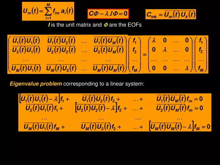
I is the unit matrix and are the EOFs Eigenvalue problemcorresponding to a linear system:
Sometimes use another complex form of EOFS. Apply the Hilbert Transformof U to understand a bit more about the phase of propagation of the phenomenon In essence, the Hilbert transform of a signal (time series) produces a complex variable with real part identical to the time series and the imaginary part is shifted 90º from the original (sometimes called the analytical signal): >> t=[1:1:1000]; >> u1=sin(2*pi*t/200); >> plot(t,u1,’LineWidth’,3) u1 t
>> t=[1:1:1000]; >> u1=sin(2*pi*t/200); >> plot(t,u1,’LineWidth’,3) >> >> u2=hilbert(u1); >> hold on; >> plot(real(u2),'r--','LineWidth',3) u t
>> t=[1:1:1000]; >> u1=sin(2*pi*t/200); >> plot(t,u1,’LineWidth’,3) >> >> u2=hilbert(u1); >> hold on >> plot(real(u2),'r--','LineWidth',3) >> plot(imag(u2),'g','LineWidth',3) u t
Hilbert Transformof U can be regarded as the convolution of U with h(t) = 1/(t) P is the Cauchy principal value (assigns values to improper integrals) • hilbert uses a four-step algorithm: • 1. It calculates the FFT of the input sequence, storing the result in a vector x. • 2. It creates a vector h whose elements h(i) have the values: • 1 for i = 1, (n/2)+1 • 2 for i = 2, 3, ... , (n/2) • 0 for i= (n/2)+2, ... , n • 3. It calculates the element-wise product of x and h. • 4. It calculates the inverse FFT of the sequence obtained in step 3 and returns the first n elements of the result.
Mean Profile 10 log (echo)
18% 60% 9%
Hilbert EOF 18% 6% 64%