Download

1 / 106
1.06k likes | 1.08k Views
This article explores linear transform techniques in multivariate data analysis, focusing on Principal Component Analysis (PCA) and Independent Component Analysis (ICA). Learn how these methods help represent and interpret complex datasets. Discover the principles behind ICA, a technique for separating independent sources from mixed data. Gain insights into statistical independence and correlation in signal processing. Explore the concepts of probability density functions, histograms, and more.

E N D
12 Microscopic Structure of Bilinear Chemical Data IASBS, Bahman 2-3, 1392 January 22-23, 2014
12 Independent Component Analysis (ICA) HadiParastar Sharif University of Technology
Every problem becomes very childish when once it is explained to you. —Sherlock Holmes (The Dancing Men, A.C. Doyle, 1905)
Representation of Multivariate Data • - The key to understand and interpret multivariate data is suitable representation • - Such a representation is achieved using some kind of transform • - Transforms can be linear or non-linear • - Linear transform W applied to a data matrix X with objects as rows and • variables as columns is as follow: • U = WX + E • - Broadly speaking, linear transform can be classified in two groups: • - Second-order methods • - Higher-order methods
Soft-modeling methods • Factor Analysis (FA) • Principal Component Analysis (PCA) • Blind source separation (BSS) • Independent Component Analysis (ICA)
hplc.m Simulating HPLC-DAD data
emgpeak.m Chromatograms with distortions
Basic statistics • Expectation • Mean • Correlation matrix
Basic statistics • Covariance matrix • Note
Principal Component Analysis (PCA) • Using an eigenvector rotation, it would be possible to decompose the X matrix into a series of loadings and scores • Underlying or intrinsic factors related to intelligence could then be detected • In chemistry, this approach can be used by diagonalizating the correlation or covariance matrix
Principal component analysis (PCA) Loadings PT Scores Raw data Residuals Data X Model TPT TPT E Noise T = + Explained variance Residual variance X=TPT+E
PCA Model: D = U VT Unexplained variance VT D E = + loadings (projections) U scores D = u1v1T + u2v2T + ……+ unvnT + E n number of components (<< number of variables in D) = + +….+ + D u1v1T u2 v2T unvnT E rank 1 rank 1 rank 1
Principal Component Analysis (PCA) x11 x12 … x114 x2 … x21 x21 x214 • • • • • • • • • • • • • • x1
u11 u2 u12 • • • • u1 • … • • • • • u114 • • • • PCA
x2 x11 x12 … x114 • • • • … x21 x21 x214 • • • • • • • • • • x1 PCA
u11 u21 u2 u1 • • u12 u22 • • … … • • u114 u214 • • • • • • • • PCA u1 = ax1 + bx2 u2 = cx1 + dx2
x1 x2 … = xn 2 x y x x . y = xTy = cos q x . y cos q = y x Inner Product (Dot Product) x . x = xTx = [x1 x2… xn] = x12 + x22 + … +xn2 The cosine of the angle of two vectors is equal to the dot product between the normalized vectors:
x y x x . y = y x y x x . y = - y y x x y = = 1 x . y = 0 Two vectors x and y are orthogonal when their scalar product is zero x . y = 0 and Two vectors x and y are orthonormal
PC2 PCA (Orthogonal coordinate) PC1 ICA (Nonorthogonal coordinate)
Independent Component Analysis: What Is It? • ICA belongs to a class of blind source separation (BSS) methods • The goal of BSS is separating data into underlying informational components, where such data can take the form of spectra, images, sounds, telecommunication channels or stock market prices. • The term “Blind” is intended to imply that such methods can separate data into source signals even if very little is known about the nature of those source signals.
The Principle of ICA: a cocktail-party problem x1(t)=a11 s1(t)+a12 s2(t)+a13 s3(t) x2(t)=a21 s1(t)+a22 s2(t) +a12 s3(t) x3(t)=a31 s1(t)+a32 s2(t) +a33 s3(t)
Independent Component Analysis Herault and Jutten, 1991 • Observed vector x is modelled by a linear latent variable model • Or in matrix form Where: --- The mixing matrix A is constant --- The si are latent variables called the independent components --- Estimate both A and s, observing only x
Independent Component Analysis • ICA bilinear model MCR model PCA model • ICA algorithms try to find independent sources
Basic properties of the ICA model • Must assume: • - The si are independent • - The si are nongaussian • - For simplicity: The matrix A is square • The si defined only up to a mltiplicative constant • The siare not ordered
lCA sources Original sources
Statistical Independence • If two or more signals are statistically independent of each other then the value of one signal provides no information regarding the value of the other signals. • For two variables • For more than two variables • Using expectation operator
Probability Density Function • Moments of probability density functions, which are essentially a form of normalized histograms. PDF Histogram Approximate of PDF
Histogram Probability
Independence and Correlation • The term “correlated” tends to be used in colloquial terms to suggest that two variables are related in a very general sense. • The entire structure of the joint pdf is implicit in the structure of its marginal pdfs because the joint pdf can be reconstructed exactly from the product of its marginal pdfs. Covariance between x and y
Marginal PDF Joint PDF
Independence and Correlation Correlation
Independence and Correlation • The formal similarity between measures of independence and correlation can be interpreted as follows: • Correlation is a measure of the amount of covariation between x and y, and depends on the first moment of the pdf p only. • Independence is a measure of the covariation between [x raised to powers p]and [y raised to powers q], and depends on all moments of the pdfpxy. • Thus, independence can be considered as a generalized measure of correlation , such that
emgpeak.m Chromatograms with distortions