Download
1 / 18
180 likes | 202 Views
Explore the problem of groundwater pollution, modeling groundwater flow and transport in aquifers, including sources of contamination and transport phenomena like dispersion and mass transport in porous media. Learn about numerical methods, aquifer properties, and forecasting groundwater quality.

E N D
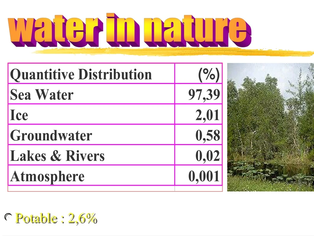
water in nature • Potable : 2,6%
Groundwater Flow • Porous media • Aquifer Properties: • T: the rate of flow per unit width through the entire thickness of an aquifer, per unit hydr. Gradient (the more great the more permeable) • S: the volume of water released from storage (or added to it) per unit horizontal area of aquifer & per unit decline (or rise) of piezometric head, φ.
GR Flow - The Problem • Darcy’s Law + Continuity (mass balance) Equation = Flow Equation (φ,T,S,x,z,y,t) • Aquifer’s Geometry • values of relevant physical coef. (K, S, ...) • Initial conditions (describe the initial state of the fluid in the domain) • Boundary cond. (how the fluid interacts with its surroundings)
GR Flow - The Solution • Analytical Methods: seldom applied • Numerical Methods (FD, FE, MOC) (Computer Revolution Aid) - Models • Forecasting Problem: to obtain φ(x,y,z,t) u(x,y,z,t)
GW Quality Problem • Quality instead of pollution (GW already contains dissolved matter) • Increasing Demand - Decreasing quality • @@% men drink unclean water ~~~ concentration of dissolved pollutants > standards by the World Health Org.
GW Pollution Sources A. Environmental • flow through carbonate rocks - dissolved rock • sea water intrusion (disturbed equillibrium) B. Domestic • accidental breaking of sewers • percolation from septic tanks • rain infiltrating through sanitary landfills • Biological contaminants (bacteria+viruses) also related to this source
GW Pollution Sources C. Industrial • a single sewage disposal for both ind.-resident. • Waste disposal in non-protected constructions • Heavy metals, toxic compounds, radioactive materials B. Agricultural • irrigation water or rain water dissolving and carrying fertilizers, salts, etc. as they infiltrate through surface and replenish the aquifer
Transport Phenomenon • Mass transport in porous media=the movement & accumulation of pollutants with the water in the interstices • 4 mechanisms affecting transport: • convection • mechanical dispersion • molecular diffusion • solid-solute interreactions, chemical reactions & decay phenomena
Dispersion • Tracer gradually spreading & occupies a region>flow domain. Irreversible process • e.g. instantaneous point injection through a well, into an aquifer - spreading (longitudinal + transversal) • ellipsoidal contours of equal concentration • breakthrough curve in obs. well (C-t)
Dispersion: reason • Mechanical Dispersion. Spread due to: • varying velocity distribution in the interstice • presence of the pore system (abnormal layout) • Molecular diffusion (low velocities) results from variations in concentr. In the liquid phase • production of an additional flux of pollutant particles from regions of higher C to those of lower ones • Mech.Disp.+Mol. Dif.=Hydrodynamic Dispersion
GW Pollution Problem • Flow equation + transport equation • Numerical methods • h(x,y,z,t) + c(x,y,z,t) • E.G. Figure : Cases of aquifer pollution
GW Flow & Transport Mathematic Models • Results • values of (x,y,z) • hydraulic heads • velocities • concentrations • value forecasting • (x,y,z,t) • aquifer’s volumetric budget Input Data • Aquifer Geometry • Boundary - Initial Conditions • Parameters • hydraulic • hydrogeologic • chemical • External stresses • Hydraulic contact (rivers-lakes-aquifers) ΜODEL