Merge and Radix Sorts

Merge and Radix Sorts Data Structures Fall, 2007 13th

Merge Sort (1/13) • Before looking at the merge sort algorithm to sort n records, let us see how one may merge two sorted lists to get a single sorted list. • Merging • The first one, Program 7.7, uses O(n) additional space. • It merges the sorted lists (list[i], … , list[m]) and (list[m+1], …, list[n]), into a single sorted list, (sorted[i], … , sorted[n]).

Merge (using O(n) space)

Merge Sort (3/13) • O(1) space merge • Steps in an O(1) space merge when the total number of records, n is a perfect square */and the number of records in each of the files to be merged is a multiple of n */ • Step1:Identify the n records with largest key. This is done by following right to left along the two files to be merged. • Step2:Exchange the records of the second file that were identified in Step1 with those just to the left of those identified from the first file so that the n record with largest keys form a contiguous block

Merge Sort (4/13) • O(1) space merge (cont’d) • Step3:Swap the block of n largest records with the leftmost block (unless it is already the leftmost block). Sort the rightmost block • Step4:Reorder the blocks excluding the block of largest records into nondecreasing order of the last key in the blocks

Merge Sort (6/13) 6, 7, 8 are merged • Step6:Sort the block with the largest keys Segment one is merged (i.e., 0, 2, 4, 6, 8, a) Change place marker (longest sorted sequence of records) Segment one is merged (i.e., b, c, e, g, i, j, k) Change place marker Segment one is merged (i.e., o, p, q) No other segment. Sort the largest keys.

When selection sort is used to implement Step 4 each block is regarded as a single record with key equal to that of the last record in the block. The time needed for these is O(n). • The total time is O(n). • The additional space used is O(1). • Example: • Input list (26, 5, 77, 1, 61, 11, 59, 15, 48, 19)

selection sort void selectionSort(int numbers[], int array_size) { int i, j; int min, temp; for (i = 0; i < array_size-1; i++) { min = i; for (j = i+1; j < array_size; j++) { if (numbers[j] < numbers[min]) min = j; } temp = numbers[i]; numbers[i] = numbers[min]; numbers[min] = temp; } } • O(n2)

Merge Sort (7/13) • Iterative merge sort • We assume that the input sequence has n sorted lists, each of length 1. • We merge these lists pairwise to obtain n/2 lists of size 2. • We then merge the n/2 lists pairwise, and so on, until a single list remains. • Analysis • Total number of passes is the celling of log2n • merge two sorted list in linear time: O(n) • The total computing time is O(n log n).

Merge Sort (8/13) • merge_pass • Invokes merge (Program 7.7) to merge the sorted sublists • Perform one pass of the merge sort. It merges adjancent pairs of subfiles from list into sorted. [0] [1] [2] [3] [4] [5] [6] [7] [8] [9] length=2 list n=10 i= 0 4 8 sorted the length of the subfile the number of elements in the list 0 4 5 1 7 3

length= 1 8 4 2 16 n=10 • merge_sort: Perform a merge sort on the file [0] [1] [2] [3] [4] [5] [6] [7] [8] [9] list extra list extra list

Merge Sort (10/13) • Recursive merge sort concept

listmerge: • Takes two sorted chains and returns an integer that points to the start of the sorted list The link field in each record is initially set to -1 Since the elements were numbered from 0 to n-1, we use list[n] to store the start pointer

lower= 5 0 5 8 9 8 5 7 1 6 5 0 4 0 3 0 2 3 0 start = rmerge(list, 0, n-1); • rmerge: sort the list, list[lower], …, list[upper]. The link field in each record is initially set to -1 upper= 4 2 9 0 1 2 9 8 4 6 9 4 7 9 7 3 6 1 5 = 0 middle= 1 2 2 0 3 4 1 2 4 7 5 4 7 8 7 6 6 5 0 0 0 8 5 3 9 6 5 3 1 2 4 7 8 list [0] [1] [2] [3] [4] [5] [6] [7] [8] [9]

Merge Sort (13/13) • Variation:Natural merge sort : • We can modify merge_sort to take into account the prevailing order within the input list. • In this implementation we make an initial pass over the data to determine the sequences of records that are in order. • The merge sort then uses these initially ordered sublists for the remainder of the passes.

Heap Sort (1/3) • The challenges of merge sort • The merge sort requires additional storage proportional to the number of records in the file being sorted. • By using the O(1) space merge algorithm, the space requirements can be reduced to O(1), but significantly slower than the original one. • Heap sort • Require only a fixed amount of additional storage • Slightly slower than merge sort using O(n) additional space • Faster than merge sort using O(1) additional space. • The worst case and average computing time is O(n log n), same as merge sort • Unstable

root = 1 n = 10 • adjust • adjust the binary tree to establish the heap rootkey = 26 child = 6 7 3 2 14 /* compare root and max. root */ [1] 77 26 /* move to parent */ 5 59 77 [2] [3] 1 61 11 26 59 [4] [5] [6] [7] 15 48 19 [8] [9] [10]

Heap Sort (3/3) • heapsort n = 10 i = 8 9 1 5 4 3 2 1 7 6 5 4 3 2 bottom-up ascending order(max heap) [1] 26 19 48 61 11 15 26 77 59 1 1 5 1 5 5 1 5 1 1 top-down 5 77 [2] 15 61 5 1 5 [3] 11 59 26 11 1 19 48 1 61 11 59 15 48 15 1 [4] [5] 19 19 5 26 1 [6] [7] 26 48 1 15 48 19 [8] 59 5 [9] 1 61 5 77 [10]

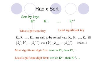
Radix Sort (1/8) • We considers the problem of sorting records that have several keys • These keys are labeled K0 (most significant key), K1, … , Kr-1 (least significant key). • Let Ki j denote key Kj of record Ri. • A list of records R0, … , Rn-1, is lexically sorted with respect to the keys K0, K1, … , Kr-1iff(Ki0, Ki1, …, Kir-1)  (K0i+1, K1i+1, …, Kr-1i+1), 0 i < n-1

Radix Sort (2/8) • Example • sorting a deck of cards on two keys, suit and face value, in which the keys have the ordering relation:K0 [Suit]:  <  <  < K1 [Face value]: 2 < 3 < 4 < … < 10 < J < Q < K < A • Thus, a sorted deck of cards has the ordering:2, …, A, … , 2, … , A • Two approaches to sort: • MSD (Most Significant Digit) first:sort on K0, then K1, ... • LSD (Least Significant Digit) first:sort on Kr-1, then Kr-2, ...

Radix Sort (3/8) • MSD first • MSD sort first, e.g., bin sort, four bins    • LSD sort second • Result: 2, …, A, … , 2, … , A

Radix Sort (4/8) • LSD first • LSD sort first, e.g., face sort, 13 bins 2, 3, 4, …, 10, J, Q, K, A • MSD sort second (may not needed, we can just classify these 13 piles into 4 separated piles by considering them from face 2 to face A) • Simpler than the MSD one because we do not have to sort the subpiles independently Result: 2, …, A, … , 2, …, A

Radix Sort (5/8) • We also can use an LSD or MSD sort when we have only one logical key, if we interpret this key as a composite of several keys. • Example: • integer: the digit in the far right position is the least significant and the most significant for the far left position • range: 0  K  999 • using LSD or MSD sort for three keys (K0, K1, K2) • since an LSD sort does not require the maintainence of independent subpiles, it is easier to implement MSD LSD 0-9 0-9 0-9

Radix Sort (6/8) • radix sort • decompose the sort key into digits using a radix r. • Ex: When r =10, we get the common base 10 or decimal decomposition of the key • LSD radix r sort • The records, R0, … ,Rn-1 • Keys: d-tuples (x0, x1, …, xd-1) and that 0  xi < r. • Each record has a link field, and that the input list is stored as a dynamically linked list. • We implement the bins as queues • front[i], 0  i < r, pointing to the first record in bin i • rear[i], 0  i < r, pointing to the last record in bin i #define MAX_DIGIT 3 /* 0 to 999 */#define RADIX_SIZE 10typedef struct list_node *list_pointer; typedef struct list_node { int key[MAX_DIGIT]; list_pointer link;};

Time complexity: O(MAX_DIGIT(RADIX_SIZE+n)) RADIX_SIZE = 10 MAX_DIGIT = 3 Initial input:179→208→306→93→859→984→55→9→271→33 MAX_DIGIT passes • LSD Radix Sort O(RADIX_SIZE) f[0] r[0] f[1] 271 r[1] O(n) NULL f[2] r[2] f[3] 93 r[3] 33 NULL f[4] r[4] 984 NULL f[5] r[5] 55 NULL f[6] r[6] 306 NULL O(RADIX_SIZE) r[7] f[7] f[8] 208 r[8] NULL f[9] 179 Chain after first pass, i=2:271→93→33→984→55→306→208→179→859→9 859 9 r[9] NULL

Radix Sort (8/8) • Simulation of radix_sort 9 f[0] r[0] Chain after second pass, i=1:306→208→9→33→55→859→271→179→984→93 Chain after third pass, i=0:9→33→55→93→179→208→271→306→859→984 f[0] 306 33 208 55 9 r[0] NULL 93 f[1] r[1] NULL f[1] 179 r[1] f[2] r[2] NULL 33 r[3] f[2] 208 f[3] NULL 271 r[2] NULL f[4] 55 f[3] r[3] 306 859 r[4] NULL NULL f[4] r[4] f[5] r[5] r[6] f[5] r[5] f[6] 271 r[7] f[6] r[6] f[7] 179 r[7] f[7] NULL r[8] 984 859 f[8] r[8] f[8] NULL NULL f[9] 93 r[9] f[9] r[9] 984 NULL NULL

Summary of Internal Sorting (1/2) • Insertion Sort • Works well when the list is already partially ordered • The best sorting method for small n • Merge Sort • The best/worst case (O(nlogn)) • Require more storage than a heap sort • Slightly more overhead than quick sort • Quick Sort • The best average behavior • The worst complexity in worst case (O(n2)) • Radix Sort • Depend on the size of the keys and the choice of the radix

Summary of Internal Sorting (2/2) • Analysis of the average running times

Merge and Radix Sorts