Understanding Self-Organizing Maps: Concepts, Algorithms, and Applications
460 likes | 585 Views
This article provides an overview of Self-Organizing Maps (SOM), a neural network algorithm developed by Teuvo Kohonen. Initially proposed in 1973, SOM utilizes unsupervised learning for data organization and visualization. It functions through a lattice of neurons that adapt their weights to input data, enabling a topographically meaningful representation. The process involves selecting a "winning" neuron and updating its weights as well as those of its neighbors. SOM has applications in various fields, including pattern recognition and data mining, despite challenges such as the need for extensive representative training data.

Understanding Self-Organizing Maps: Concepts, Algorithms, and Applications
E N D
Presentation Transcript
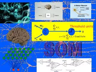
x0 w0 Threshold units o xn wn SOM
Neurons Inputs Teuvo Kohonen
Self-Organizing Maps : Origins • Ideas first introduced by C. von der Malsburg (1973), developed and refined by T. Kohonen (1982) • Neural network algorithm using unsupervised competitive learning • Primarily used for organization and visualization of complex data • Biological basis: ‘brain maps’
j 2d array of neurons Weighted synapses wj1 wj2 wj3 wjn Set of input signals (connected to all neurons in lattice) x1 x2 x3 ... xn Self-Organizing Maps SOM - Architecture • Lattice of neurons (‘nodes’) accepts and responds to set of input signals • Responses compared; ‘winning’ neuron selected from lattice • Selected neuron activated together with ‘neighbourhood’ neurons • Adaptive process changes weights to more closely resemble inputs
Self-Organizing Maps SOM – Algorithm Overview Randomly initialise all weights Select input vector x = [x1, x2, x3, … , xn] Compare x with weights wj for each neuron j to determine winner Update winner so that it becomes more like x, together with the winner’s neighbours Adjust parameters: learning rate & ‘neighbourhood function’ Repeat from (2) until the map has converged (i.e. no noticeable changes in the weights) or pre-defined no. of training cycles have passed
Initialisation Randomly initialise the weights
Finding a Winner • Find the best-matching neuron w(x), usually the neuron whose weight vector has smallestEuclideandistance from the input vector x • The winning node is that which is in some sense ‘closest’ to the input vector • ‘Euclidean distance’ is the straight line distance between the data points, if they were plotted on a (multi-dimensional) graph • Euclidean distance between two vectors a and b, • a = (a1,a2,…,an), b = (b1,b2,…bn), is calculated as: Euclidean distance
L. rate No. of cycles Weight Update • SOM Weight Update Equation • wj(t +1) = wj(t) + (t)(x)(j,t)[x - wj(t)] • “The weights of every node are updated at each cycle by adding • Current learning rate × Degree of neighbourhood with respect to winner × Difference between current weights and input vector • to the current weights” • Example of (t) Example of (x)(j,t) • x-axis shows distance from winning node • y-axis shows ‘degree of neighbourhood’ (max. 1)
Kohonen’s Algorithm jth input Winner ith
Neighborhoods Square and hexagonal grid with neighborhoods based on box distance Grid-lines are not shown
i • i • Neighborhood of neuron i • One-dimensional • Two-dimensional
position of k position of i • A neighborhood function (i, k) indicates how closely neurons i and k in the output layer are connected to each other. • Usually, a Gaussian function on the distance between the two neurons in the layer is used:
A simple toy example Clustering of the Self Organising Map
However, instead of updating only the winning neuron i*, all neurons within a certain neighborhood Ni* (d), of the winning neuron are updated using the Kohonen rule. Specifically, we adjust all such neurons iNi* (d), as follow Here the neighborhood Ni* (d), contains the indices for all of the neurons that lie within a radius d of the winning neuron i*.
Topologically Correct Maps The aim of unsupervised self-organizing learning is to construct a topologically correct map of the input space.
i i w w After learning Before learning Self Organizing Map • Determine the winner (the neuron of which the weight vector has the smallest distance to the input vector) • Move the weight vector w of the winning neuron towards the input i
Network Features • Input nodes are connected to every neuron • The “winner” neuron is the one whose weights are most “similar” to the input • Neurons participate in a “winner-take-all” behavior • The winner output is set to 1 and all others to 0 • Only weights to the winner and its neighbors are adapted
wi P 1 2 3 4 5 6 7 8 9
5 wi2 6 4 3 9 7 P2 P1 2 1 8 wi1
winner output input (n-dimensional)
0 20 100 1000 10000 25000 Example I: Learning a one-dimensional representation of a two-dimensional (triangular) input space:
Self Organizing Map • Impose a topological order onto the competitive neurons (e.g., rectangular map) • Let neighbors of the winner share the “prize” (The “postcode lottery” principle) • After learning, neurons with similar weights tend to cluster on the map
Conclusion • Advantages • SOM is Algorithm that projects high-dimensional data onto a two-dimensional map. • The projection preserves the topology of the data so that similar data items will be mapped to nearby locations on the map. • SOM still have many practical applications in pattern recognition, speech analysis, industrial and medical diagnostics, data mining • Disadvantages • Large quantity of good quality representative training data required • No generally accepted measure of ‘quality’ of a SOM • e.g. Average quantization error (how well the data is classified)
Topologies (gridtop, hextop, randtop) pos = gridtop(3,2) pos = 0 1 0 1 0 1 0 0 1 1 2 2 plotsom(pos) pos = gridtop(2,3) pos = 0 1 0 1 0 1 0 0 1 1 2 2 plotsom(pos)
pos = gridtop(8,10); plotsom(pos)
pos = hextop(2,3) pos = 0 1.0000 0.5000 1.5000 0 1.0000 0 0 0.8660 0.8660 1.7321 1.7321
pos = hextop(3,2) pos = 0 1.0000 2.0000 0.5000 1.5000 2.5000 0 0 0 0.8660 0.8660 0.8660 plotsom(pos)
pos = hextop(8,10); plotsom(pos)
pos = randtop(2,3) pos = 0 0.7787 0.4390 1.0657 0.1470 0.9070 0 0.1925 0.6476 0.9106 1.6490 1.4027
pos = randtop(3,2) pos = 0 0.7787 1.5640 0.3157 1.2720 2.0320 0.0019 0.1944 0 0.9125 1.0014 0.7550
pos = randtop(8,10); plotsom(pos)
Distance Funct. (dist, linkdist, mandist, boxdist) pos2 = [ 0 1 2; 0 1 2] pos2 = 0 1 2 0 1 2 D2 = dist(pos2) D2 = 0 1.4142 2.8284 1.4142 0 1.4142 2.8284 1.4142 0
pos = gridtop(2,3) pos = 0 1 0 1 0 1 0 0 1 1 2 2 plotsom(pos) d = boxdist(pos) d = 0 1 1 1 2 2 1 0 1 1 2 2 1 1 0 1 1 1 1 1 1 0 1 1 2 2 1 1 0 1 2 2 1 1 1 0
pos = gridtop(2,3) pos = 0 1 0 1 0 1 0 0 1 1 2 2 plotsom(pos) d=linkdist(pos) d = 0 1 1 2 2 3 1 0 2 1 3 2 1 2 0 1 1 2 2 1 1 0 2 1 2 3 1 2 0 1 3 2 2 1 1 0
The Manhattan distance between two vectors x and y is calculated as D = sum(abs(x-y)) Thus if we have W1 = [ 1 2; 3 4; 5 6] W1 = 1 2 3 4 5 6 and P1= [1;1] P1 = 1 1 then we get for the distances Z1 = mandist(W1,P1) Z1 = 1 5 9
A One-dimensional Self-organizing Map angles = 0:2*pi/99:2*pi; P = [sin(angles); cos(angles)]; plot(P(1,:),P(2,:),'+r')
net = newsom([-1 1;-1 1],[30]); net.trainParam.epochs = 100; net = train(net,P); plotsom(net.iw{1,1},net.layers{1}.distances) The map can now be used to classify inputs, like [1; 0]: Either neuron 1 or 10 should have an output of 1, as the above input vector was at one end of the presented input space. The first pair of numbers indicate the neuron, and the single number indicates its output. p = [1;0]; a = sim (net, p) a = (1,1) 1
x = -4:0.01:4 P = [x;x.^2]; plot(P(1,:),P(2,:),'+r') net = newsom([-10 10;0 20],[10 10]); net.trainParam.epochs = 100; net = train(net,P); plotsom(net.iw{1,1},net.layers{1}.distances)