Download
1 / 45
450 likes | 556 Views
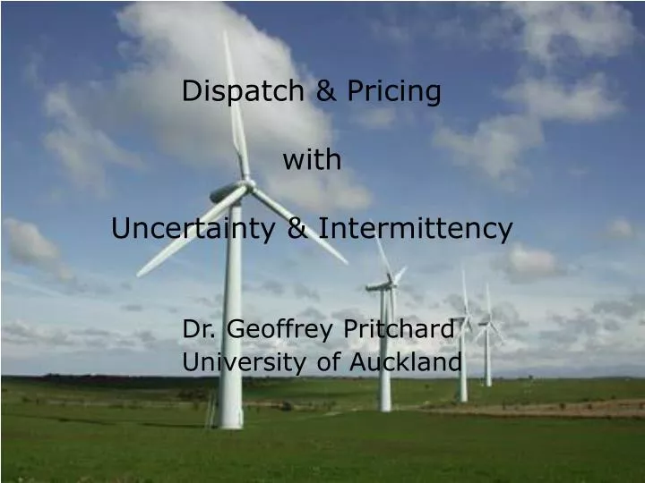
Dispatch & Pricing with Uncertainty & Intermittency. Dr. Geoffrey Pritchard University of Auckland. NZ has a large wind resource. 500 MW now installed or committed. many more sites under investigation or seeking consents. 3000+ MW potential

E N D
Dispatch & Pricing with Uncertainty & Intermittency Dr. Geoffrey Pritchard University of Auckland
NZ has a large wind resource • 500 MW now installed or committed. • many more sites under investigation or seeking consents. • 3000+ MW potential • but this ignores system integration issues.
Wind is unpredictable and variable • Wind forecast error exceeds load forecast error in NI with >370 MW wind. (WGIP, 2 hour forecasts, 1-month return period events) • Wind variability is about half of load variability in NI with 1600 MW wind. (WGIP, 10 sec or 5 min periods, 1-month return period events)
Accommodating uncertainty (wind and load) • Processes: • 5-minute re-dispatch • Frequency-keeping • Technologies: • Hydro • Fast gas turbine • Responsive loads (EV battery charging?)
Wind/hydro matching • Why not pair off each wind farm with a hydro? • transmission implications if not co-located. • doesn’t make full use of hydro flexibility. • doesn’t allow wind farms to match with each other. • Matching might be done better at the power system level.
The dispatch process (at present) -2hr 0 +30min • Generator offers close • Loads, wind forecast • SPD run to find optimal dispatch • Actual loads, wind • SPD re-dispatch every 5 min • Frequency-keepers adjust continuously
Could the system operation / market be extended to treat uncertainty optimally?
Example Wind: 100 forecast, @ $0 Thermal A: 400 @ $45 Capacity 250 lossless Hydro: 200 @ $30, 200 @ $90 Thermal B: 400 @ $50 Load 500 • Wind forecast may be inaccurate. • Hydro can be re-dispatched in response, thermals can’t. • What to dispatch?
Least-(forecast)-cost dispatch 100 150 Wind: 100 forecast, @ $0 Thermal A: 400 @ $45 250 Capacity 250 lossless Hydro: 200 @ $30, 200 @ $90 200 50 Thermal B: 400 @ $50 Load 500 The best solution, on the assumption that the wind forecast is accurate.
Wind above forecast 100 150 Wind: 120 actual, @ $0 Thermal A: 400 @ $45 spill 20 250 Capacity 250 lossless Hydro: 200 @ $30, 200 @ $90 200 50 Thermal B: 400 @ $50 Load 500 Wind is spilled – cheap energy is lost.
Wind below forecast 80 150 Wind: 80 actual, @ $0 Thermal A: 400 @ $45 230 Capacity 250 lossless Hydro: 200 @ $30, 200 @ $90 220 50 Thermal B: 400 @ $50 Load 500 Wind shortfall is made up with expensive water.
Better forecasting? • Forecast errors in either direction incur high penalties • so smaller errors would certainly help. • Can the penalties themselves be reduced?
Hedging vs. uncertainty 100 125 Wind: 100 forecast, @ $0 Thermal A: 400 @ $45 225 Capacity 250 lossless Hydro: 200 @ $30, 200 @ $90 175 100 Thermal B: 400 @ $50 Load 500 • Spare capacity on transmission line. • Spare capacity in cheap hydro tranche.
Wind above forecast 120 125 Wind: 120 actual, @ $0 Thermal A: 400 @ $45 245 Capacity 250 lossless Hydro: 200 @ $30, 200 @ $90 155 100 Thermal B: 400 @ $50 Load 500 Surplus wind is matched to hydro.
Wind below forecast 80 125 Wind: 80 actual, @ $0 Thermal A: 400 @ $45 205 Capacity 250 lossless Hydro: 200 @ $30, 200 @ $90 195 100 Thermal B: 400 @ $50 Load 500 Surplus wind is matched to hydro.
Hedged vs. conventional dispatch 100 125 (25 less) Wind: 100 forecast, @ $0 Thermal A: 400 @ $45 225 (25 less) Capacity 250 lossless Hydro: 200 @ $30, 200 @ $90 175 (25 less) 100 (50 more) Thermal B: 400 @ $50 Load 500 • Adjustment Thermal A ->Thermal B costs $5, • but allows chance to save water worth $30. • Adjustment Hydro ->Thermal B costs $20, • but allows chance to save $60 on water.
Is the hedged dispatch better? • Depends on the probabilities involved. • The more uncertainty in the wind, the more hedging will be worthwhile.
Allowing for uncertainty in one offer (or load) affects the dispatch of other offers, even those that are not uncertain themselves.
What not to conclude from the example • Hedged dispatch means higher thermal fuel burn. • Other, similar examples adjust dispatch away from thermals. • The transmission network is the essential element. • Other, similar examples have one node, no lines.
Could the system operation / market be extended to treat uncertainty optimally?
Market principles “There is only one market” • No separate day-ahead and regulating market • (as in Nordpool etc.) • No separate markets for ancillary services. • Exception: the present frequency-keeping auction. • Not an exception: instantaneous reserve (co-optimized). • A generator shouldn’t have to choose which market to offer into. • Potential arbitrage, illiquidity, market power issues.
Instantaneous reserve • IR is insurance against truly rare events. • Includes the effect of exceptional weather on wind farms • But not most wind fluctuations.
Optimizing dispatch (conventional) Generators offer to sell tranches qi, ask prices pi We find dispatches xi to minimize Spi xi (cost of power, at offered prices) so that • demand is met • transmission network is operated within capacity • 0 < xi < qi
Optimizing dispatch (hedged) One approach: Generators offer to sell tranches qi, asking prices pi We find dispatches • xi (1st stage: initial dispatch) • Zi (2nd stage: real-time, contingent on random events) Three kinds of offer: • Inflexible (“thermal”), no re-dispatching, Zi = xi • Flexible (“hydro”), arbitrary re-dispatching, 0< xi < qi, 0< Zi < qi • Intermittent (“wind”), 0< xi < qi, 0< Zi < Si (random)
Optimizing dispatch (hedged) Generators offer to sell tranches qi, ask prices pi Flexible plant may also offer • to sell additional power via re-dispatch, ask pricepi +ri • to buy back power via re-dispatch, bid price pi -ri where ri is a regulation margin.
Optimizing dispatch (hedged) Generators offer to sell tranches qi , ask prices pi ,regulation margins ri We find dispatches xi and Zi to minimize S (pi xi + E[ (pi +ri)(Zi - xi)+ - (pi -ri)(Zi - xi)- ] ) (expected cost of power, at offered prices, including re-dispatch) so that • demand is met (at both 1st and 2nd stages) • transmission network is operated within capacity • (xi , Zi ) satisfy plant constraints
Example Wind: capacity 40, @ $0 scenarios0, 10, 20, 30 probabilities0.5, 0.2, 0.2, 0.1 Hydro 1: 40 @ $39 (+/- $2) Hydro 2: 40 @ $40 (+/- $5) Load 60 • Ensemble forecast for wind. Most likely scenario is 0. • Hydros compete on both energy and regulation. • What to dispatch?
Optimal hedged dispatch (initial) Wind: capacity 40, @ $0 scenarios0, 10, 20, 30 probabilities0.5, 0.2, 0.2, 0.1 30 Hydro 1: 40 @ $39 (+/- $2) 10 20 Hydro 2: 40 @ $40 (+/- $5) Load 60 • Hydros dispatched “out of order” to keep regulation cost down.
Optimal hedged re-dispatch Wind: capacity 40, @ $0 scenarios0, 10, 20, 30 probabilities0.5, 0.2, 0.2, 0.1 Hydro 1: 40 @ $39 (+/- $2) 0, 10, 20, 30 40, 30, 20, 10 Hydro 2: 40 @ $40 (+/- $5) 20 Load 60 • Hydro 1 wins the regulation business.
Market pricing (conventional) • Conventional spot price: the marginal cost of a unit of additional load. • This is an appropriate price at which to trade spot energy. • This already varies by • location (in the network) • time (of day).
Market pricing (hedged) • We have now introduced an economic distinction between initial dispatch and re-dispatch.
Initial dispatch prices • pn – the marginal cost of an additional unit of load at node n in the initial dispatch. • This is an appropriate price at which to trade energy, where that energy was present in the initial dispatch. • Applies to: • inflexible load and generation • some flexible and intermittent generation
Re-dispatch prices • pnR – the marginal cost of an additional unit of load at node n in a re-dispatch. • This is an appropriate price at which to trade energy, where that energy was added in a re-dispatch. • Applies to: • some flexible and intermittent generation (both hydro & wind)
Example: initial dispatch prices Wind: capacity 40, @ $0 scenarios0, 10, 20, 30 probabilities0.5, 0.2, 0.2, 0.1 30 Hydro 1: 40 @ $39 (+/- $2) 10 20 Hydro 2: 40 @ $40 (+/- $5) $40 Load 60 • Marginal additional load would be met by Hydro 2. • The quantities xi are sold @ $40; load pays $40.
Example: re-dispatch prices Wind: capacity 40, @ $0 scenarios0, 10, 20, 30 probabilities0.5, 0.2, 0.2, 0.1 Hydro 1: 40 @ $39 (+/- $2) 0, 10, 20, 30 40, 30, 20, 10 Hydro 2: 40 @ $40 (+/- $5) 20 $41, $41, $37, $37 Load 60 • 1st scenario: Wind buys back 10 @ $41; Hydro 1 sells 10 @ $41 • 2nd scenario: no re-dispatch • 3rd scenario: Wind sells 10 @ $37; Hydro 1 buys back 10 @ $37 • 4th scenario: Wind sells 20 @ $37; Hydro 1 buys back 20 @ $37
Average selling prices Wind: capacity 40, @ $0 scenarios0, 10, 20, 30 probabilities0.5, 0.2, 0.2, 0.1 Hydro 1: 40 @ $39 (+/- $2) 0, 10, 20, 30 40, 30, 20, 10 Hydro 2: 40 @ $40 (+/- $5) 20 $41, $41, $37, $37 Load 60 • Average selling price achieved • = (expected revenue) / (expected generation) • Wind: $38.11 • Hydro 1: $40.55 • Hydro 2: $40
Example: multiple wind farms Wind 1: capacity 100, @ $0 scenarios40, 40, 45, 55, 50, 50, 50, 60 Thermal: 100 @ $58 Hydro: 30 @ $40 (+/- $4) 60 @ $60 (+/- $4) Wind 2: capacity 100, @ $0 scenarios40, 50, 50, 60, 50, 55, 60, 60 Wind 3: capacity 100, @ $0 scenarios45, 50, 60, 50, 45, 55, 40, 55 Load 300 equally likely scenarios
Correlations between wind farms Wind 2 Wind 3 Wind 3 Wind 1 Wind 2 Wind 1 • Wind 1 and Wind 2 are somewhat correlated • Wind 3 is relatively uncorrelated
Initial dispatch Wind 1: capacity 100, @ $0 scenarios40, 40, 45, 55, 50, 50, 50, 60 95 Thermal: 100 @ $58 50 Hydro: 30 @ $40 (+/- $4) 60 @ $60 (+/- $4) 50 $58 Wind 2: capacity 100, @ $0 scenarios40, 50, 50, 60, 50, 55, 60, 60 55 50 Wind 3: capacity 100, @ $0 scenarios45, 50, 60, 50, 45, 55, 40, 55 Load 300 equally likely scenarios • Hydro is dispatched ahead of thermal to facilitate regulation. • Thermal is marginal at $58. • In some scenarios, the wind farms can trade with each other. • Average overall selling prices achieved: • Thermal $58, Hydro $59.01, • Wind 1 $57.54, Wind 2 $57.60, Wind 3 $57.80
Revenue adequacy • Conventional: (Total payments received from loads) minus (Total payments to generators) gives a non-negative surplus. (Loss & constraint rental.) • The same is true with optimal hedged dispatch and re-dispatch pricing, in all scenarios.
Another example Thermal 2: 100 @ $45 Wind 2: 60 @ $0 Wind 1: 60 @ $0 Hydro: 50 @ $42 (+/- $10) 60 @ $80 (+/- $10) Thermal 1: 100 @ $40 capacity 150 Load 264 Wind farms treated as deterministic (i.e. accurately forecast).
Conventional dispatch Thermal 2: 100 @ $45 0 60 Wind 2: 60 @ $0 60 Wind 1: 60 @ $0 $41 $40.5 $41.5 99 Hydro: 50 @ $42 (+/- $10) 60 @ $80 (+/- $10) Thermal 1: 100 @ $40 45 $40 $42 $42.5 capacity 150 Load 264 Spring washer effect – a very constrained solution.
Hedged version of the problem Thermal 2: 100 @ $45 Wind 1: capacity 100, @ $0 scenarios30, 50, 60, 70, 90 equally likely Wind 2: capacity 100, @ $0 scenarios30, 50, 60, 70, 90 equally likely Hydro: 50 @ $42 (+/- $10) 60 @ $80 (+/- $10) Thermal 1: 100 @ $40 capacity 150 Wind farms independent Load 264 Ensemble forecast for wind farms. Note 60 is still the best forecast for each wind farm.
Hedged dispatch and pricing Thermal 2: 100 @ $45 45 (45 more) Wind 1: capacity 100, @ $0 scenarios30, 50, 60, 70, 90 equally likely Wind 2: capacity 100, @ $0 scenarios30, 50, 60, 70, 90 equally likely 60 60 $45 $42.5 $47.5 69 (30 less) Hydro: 50 @ $42 (+/- $10) 60 @ $80 (+/- $10) Thermal 1: 100 @ $40 $40 $50 $52.5 capacity 150 30 (15 less) Load 264 • Hydro dispatch is reduced to avoid the risk of using $80 water. • Line is not at capacity (it carries 145) • - this facilitates regulation by maintaining flexibility. • Prices anticipate a possible spring-washer upon re-dispatch.
Dispatch & Pricing with Uncertainty & Intermittency Dr. Geoffrey Pritchard University of Auckland