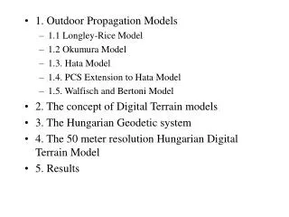
Outdoor Propagation Model
Outdoor Propagation Model. For macrocell. Okumura Model. wholly based on measured data - no analytical explanation among the simplest & best for in terms of path loss accuracy in cluttered mobile environment disadvantage : slow response to rapid terrain changes

Outdoor Propagation Model
E N D
Presentation Transcript
Outdoor Propagation Model For macrocell
Okumura Model • wholly based on measured data - no analytical explanation • among the simplest & best for in terms of path loss accuracy in cluttered mobile environment • disadvantage: slow response to rapid terrain changes • common std deviations between predicted & measured path loss 10dB - 14dB • widely used for urban areas • useful for • frequencies ranging from 150MHz-1920MHz • frequencies can be extrapolated to 3GHz • distances from 1km to 100km • base station antenna heights from 30m-1000m
Okumura Model • Okumura developed a set of curves in urban areas with quasi-smooth terrain • effective antenna height: • base station hte = 200m • mobile: hre= 3m • gives median attenuation relative to free space (Amu) • developed from extensive measurements using vertical omni- directional antennas at base and mobile • measurements plotted against frequency
Estimating path loss using Okumura Model • 1. determine free space lossLF, between points of interest • 2. add Amu(f,d) and correction factors to account for terrain L50(dB)= LF + Amu(f,d) – G(hte) – G(hre) – GAREA L50 = 50% value of propagation path loss (median) LF = free space propagation loss Amu(f,d) = median attenuation relative to free space G(hte) = base station antenna height gain factor G(hre) = mobile antenna height gain factor GAREA = gain due to environment
Estimating path loss using Okumura Model • Four steps: • a) calculate free-space path loss at the considered distance and carrier frequency • b) add median attenuation at the considered distance and carrier frequency • c) subtract the TX and RX antenna gains (see following formulas) • d) subtract the gain due to the specific environment.The values of Aμ(fc, d) and GAREA are obtained fromOkumura empirical plots
G(hte) = 10m < hte< 1000m hre 3m G(hre) = G(hre) = 3m < hre <10m Estimating path loss using Okumura Model • model corrected for • - h = terrain undulation height • - isolated ridge height • - average terrain slope • - mixed land/sea parameter
Okumura-Hata model cont. • 3 types of prediction area : • Open area : open space, no tall trees or building in path • Suburban area : Village Highway scattered with trees and house. Some obstacles near the mobile but not very congested • Urban area : Built up city or large town with large building and houses. Village with close houses and tall
Hata Model • empirical model of graphical path loss data from Okumura • predicts median path loss for different channels • valid over UHF/VHF band from 150MHz-1.5GHz • charts used to characterize factors affecting mobile land propagation • standard formulas for approximating urban propagation loss • correction factors for some situations • compares closely with Okumura model as d > 1km large mobile systems • incorporates the graphical information from Okumura model and develops it further to realize the effects of diffraction, reflection and scattering caused by city structures
Hata Model cont… L50 (urban)(dB) = 69.55 + 26.16log10 fc– 13.82 log10 the– (hre) + (44.9-6.55hte)log10 d
Hata Model for Rural and Suburban Regions represent reductions in fixed losses for less demanding environments Mobile Antenna Height Correction Factor for Hata Model
for medium sized cities CM = 0dB metropolitan centers CM = 3dB PCS Extension to Hata Model extend Hata model to 2GHz L50 (urban)(dB) = 46.3 + 33.9logfc– 13.82 loghte – (hre) + (44.9-6.55hte)logd + CM fc = frequency from 1500MHz - 2 GHz hte = 30m-200m hre = 1m-10m d = 1km-20km
Example 5 • Suppose you received a license to operate at frequency of 1.7 GHz transmitting 5W into a 10dB gain antenna at a height of 30m above the ground. Your portable receiver having an antenna gain of 2dB and height of 1m above the ground level. The portable receiver can be used at a distance of 5km from base station. With this information and using charts from Okumura model estimate the received signal at portable receiver for urban, suburban and open area.
Example 6 • Find the median path loss using Okumura’s model for d =50 km, hte=100m, hre=10m in a suburban environment. If the base station transmitter radiates an EIRP of 1kW at a carrier frequency of 900MHz, find the power at the receiver(assume a unity gain receiving antenna).