Automatic Algorithm Configuration based on Local Search
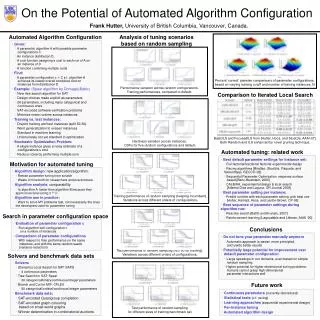
This presentation discusses the automation of algorithm tuning processes, focusing on developing the best parameter configurations for solving complex problems. Manual tuning is often time-intensive, consuming up to 50% of development time. The proposed solution leverages statistical optimization methods, such as Iterated Local Search (ILS), to efficiently explore the parameter space and find optimal configurations. The research addresses various application areas, including NP-hard problems, computer vision, and supervised machine learning, aiming to improve performance while simplifying the tuning process.

Automatic Algorithm Configuration based on Local Search
E N D
Presentation Transcript
Automatic Algorithm Configuration based on Local Search EARG presentationDecember 13, 2006 Frank Hutter
Motivation • Want to design “best” algorithm A to solve a problem • Many design choices need to be made • Some choices deferred to later: free parameters of algorithm • Set parameters to maximise empirical performance • Finding best parameter configuration is non-trivial • Many parameter configurations • Many test instances • Many runs to get realistic estimates for randomised algorithms • Tuning still often done manually, up to 50% of development time • Let’s automate tuning!
Parameters in different research areas • NP-hard problems: tree search • Variable/value heuristics, learning, restarts, … • NP-hard problems: local search • Percentage of random steps, tabu length, strength of escape moves, … • Nonlinear optimisation: interior point methods • Slack, barrier init, barrier decrease rate, bound multiplier init, … • Computer vision: object detection • Locality, smoothing, slack, … • Compiler optimisation, robotics, … • Supervised machine learning • NOT model parameters • L1/L2 loss, penalizer, kernel, preprocessing, num. optimizer, …
Related work • Best fixed parameter setting • Search approaches [Minton ’93, ‘96], [Hutter ’04], [Cavazos & O’Boyle ’05],[Adenso-Diaz & Laguna ’06], [Audet & Orban ’06] • Racing algorithms/Bandit solvers [Birattari et al. ’02], [Smith et al. ’04 – ’06] • Stochastic Optimisation [Kiefer & Wolfowitz ’52], [Geman & Geman ’84], [Spall ’87] • Per instance • Algorithm selection [Knuth ’75], [Rice 1976], [Lobjois and Lemaître ’98], [Leyton-Brownet al. ’02], [Gebruers et al. ’05] • Instance-specific parameter setting [Patterson & Kautz ’02] • During algorithm run • Portfolios [Kautz et al. ’02], [Carchrae & Beck ’05], [Gagliolo & Schmidhuber ’05, ’06] • Reactive search[Lagoudakis & Littman ’01, ’02], [Battiti et al ’05], [Hoos ’02]
Static Algorithm Configuration (SAC) SAC problem instance: 3-tuple (D,A,Q), where • D is a distribution of problem instances, • A is a parameterised algorithm, and • Q is the parameter configuration space of A. Candidate solution: configuration q2Q, expected cost C(q) = EI»D[Cost(A, q, I)] • Stochastic Optimisation Problem
Static Algorithm Configuration (SAC) SAC problem instance: 3-tuple (D,A,Q), where • D is a distribution of problem instances, • A is a parameterised algorithm, and • Q is the parameter configuration space of A. CD(A, q, D): cost distribution of algorithm A with parameterconfiguration q across instances from D. Variation due to randomisation of A and variation in instances. Candidate solution: configuration q2Q, expected cost C(q) = statistic[ CD(A, q, I) ] • Stochastic Optimisation Problem
Parameter tuning in practice • Manual approaches are often fairly ad hoc • Full factorial design • Expensive (exponential in number of parameters) • Tweak one parameter at a time • Only optimal if parameters independent • Tweak one parameter at a time until no more improvement possible • Local search ! local minimum • Manual approaches are suboptimal • Only find poor parameter configurations • Very long tuning time • Want to automate
What is the objective function? • User-defined objective function • E.g. expected runtime across a number of instances • Or expected speedup over a competitor • Or average approximation error • Or anything else • BUT: must be able to approximate objective based on a finite (small) number of samples • Statistic is expectation ! sample mean (weak law of large numbers) • Statistic is median ! sample median (converges ??) • Statistic is 90% quantile ! sample 90% quantile (underestimated with small samples !) • Statistic is maximum (supremum) ! cannot generally approximate based on finite sample?
Parameter tuning as “pure” optimisation problem • Approximate objective function (statistic of a distribution) based on fixed number of N instances • Beam search [Minton ’93, ‘96] • Genetic algorithms [Cavazos & O’Boyle ’05] • Exp. design & local search [Adenso-Diaz & Laguna ‘06] • Mesh adaptive direct search [Audet & Orban ‘06] • But how large should N be ? • Too large: take too long to evaluate a configuration • Too small: very noisy approximation ! over-tuning
Minimum is a biased estimator • Let x1, …, xn be realisations of rv’s X1, …, Xn • Each xi is a priori an unbiased estimator of E[ Xi ] • Let xj = min(x1,…,xn) This is an unbiased estimator of E[ min(X1,…,Xn) ]but NOT of E[ Xj ] (because we’re conditioning on it being the minimum!) • Example • Let Xi» Exp(l), i.e. F(x|l) = 1 - exp(-lx) • E[ min(X1,…,Xn) ] = 1/n E[ min(Xi) ] • I.e. if we just take the minimum and report its runtime, we underestimate cost by a factor of n (over-confidence) • Similar issues for cross-validation etc
Primer: over-confidence for N=1 sample y-axis: runlength of best q found so far Training: approximation based on N=1 sample (1 run, 1 instance) Test: 100 independent runs (on the same instance) for each q Median & quantiles over 100 repetitions of the procedure
Over-tuning • More training ! worse performance • Training cost monotonically decreases • Test cost can increase • Big error in cost approximation leads to over-tuning (on expectation): • Let q* 2Q be the optimal parameter configuration • Let q’ 2Q be a suboptimal parameter configuration with better training performance than q* • If the search finds q* before q’ (and it is the best one so far), and the search then finds q’, training cost decreases but test cost increases
Other approaches without over-tuning • Another approach • Small N for poor configurations q, large N for good ones • Racing algorithms [Birattari et al. ’02, ‘05] • Bandit solvers [Smith et al., ’04 –’06] • But treat all parameter configurations as independent • May work well for small configuration spaces • E.g. SAT4J has over a million possible configurations! Even a single run each is infeasible • My work: combination of approaches • Local search in parameter configuration space • Start with N=1 for each q, increase it whenever q re-visited • Does not have to visit all configurations, good ones visited often • Does not suffer from over-tuning
Unbiased ILS in parameter space • Over-confidence for each q vanishes as N!1 • Increase N for good q • Start with N=0 for all q • Increment N for qwhenever q is visited • Can proof convergence • Simple property, even applies for round-robin • Experiments: SAPS on qwh ParamsILS with N=1 Focused ParamsILS
SAC problem instances • SAPS [Hutter, Tompkins, Hoos ’02] • 4 continuous parameters ha,r,wp, Psmoothi • Each discretised to 7 values ! 74 =2,401configurations • Iterated Local Search for MPE [Hutter ’04] • 4 discrete + 4 continuous (2 of them conditional) • In total 2,560 configurations • Instance distributions • Two single instances, one easy (qwh), one harder (uf) • Heterogeneous distribution with 98 instances from satlib for which SAPS median is 50K-1M steps • Heterogeneous distribution with 50 MPE instances: mixed • Cost: average runlength, q90 runtime, approximation error
Local Search for SAC: Summary • Direct approach for SAC • Positive • Incremental homing-in to good configurations • But using the structure of parameter space (unlike bandits) • No distributional assumptions • Natural treatment of conditional parameters • Limitations • Does not learn • Which parameters are important? • Unnecessary binary parameter: doubles search space • Requires discretization • Could be relaxed (hybrid scheme etc)

