Download
1 / 38
380 likes | 500 Views
1 st level analysis: Design matrix, contrasts, and inference Roy Harris & Caroline Charpentier. Outline. A B C D. [1 -1 -1 1]. What is ‘ 1st level analysis ’? The Design matrix What are we testing for? What do all the black lines mean?

E N D
1st level analysis: Design matrix, contrasts, and inferenceRoy Harris & Caroline Charpentier
Outline A B C D [1 -1 -1 1] • What is ‘1st level analysis’? • The Design matrix • What are we testing for? • What do all the black lines mean? • What do we need to include? • Contrasts • What are they for? • t and F contrasts • How do we do that in SPM8? • Levels of inference
Overview StatisticalParametricMap Designmatrix fMRItime-series kernel Motion correction Smoothing General Linear Model ParameterEstimates Spatial normalisation Standard template • Once the image has been reconstructed, realigned, spatially normalised and smoothed…. • The next step is to statistically analyse the data Rebecca Knight
Key concepts • 1st level analysis – A within subjects analysis where activation is averaged across scans for an individual subject • The Between - subject analysis is referred to as a 2nd level analysisand will be described later on in this course • Design Matrix–The set of regressors that attempts to explain the experimental data using the GLM A dark-light colour map is used to show the value of each variable at specific time points – 2D, m = regressors, n = time. • The Design Matrixforms part of theGeneral linear model, the majority of statistics at the analysis stage use the GLM
General Linear Model Generic Model β ε + Y X x = Dependent Variable (What you are measuring) Independent Variable (What you are manipulating) Relative Contributionof X to the overalldata (These need tobe estimated) Error (The difference between the observed data and that which is predicted by the model) • Aim: To explain as much of the variance in Y by using X, and thus reducing ε Y = X1β1 + X2β2 + ....X nβn.... + ε
GLM continued • How does this equation translate to the1st level analysis ? • Each letter is replaced by a set ofmatrices(2D representations) β X Y + ε x = Matrix of BOLDat various time points in a single voxel (What you collect) Design matrix (This is your model specification in SPM) Parameters matrix (These need to be estimated) Error matrix (residual error for each voxel) Parameter weights (rows) Time (rows) Time (rows) Time(rows) 1 x column (Voxel) Regressors (columns) 1 x Column
‘Y’ in the GLM Y Y = Matrix of Bold signals Voxel time course fMRI brain scans Time Time (scan every 3 seconds) 1 voxel = ~ 3mm³ Amplitude/Intensity Rebecca Knight
‘X’ in the GLM X = Design Matrix Time (n) Regressors (m)
Regressors • Regressors– represent the hypothesised contribution of your experiment to the fMRI time series. They are represented by the columns in the design matrix (1column = 1 regressor) • Regressors of interesti.e. Experimental Regressors– represent those variables which you intentionally manipulated. The type of variable used affects how it will be represented in the design matrix • Regressorsof no interestor nuisance regressors – represent those variables which you did not manipulate but you suspect may have an effect. By including nuisance regressors in your design matrix you decrease the amount of error. • E.g. -The 6movement regressors (rotations x3 & translations x3 ) or physiological factors e.g. heart rate, breathing or others (e.g., scanner known linear drift)
Conditions • Termed indicator variables as they indicate conditions • Type of dummy code is used to identify the levels of each variable • E.g. Two levels of one variable is on/off, represented as ON = 1 OFF = 0 Changes in the bold activation associated with the presentation of a stimulus When you IV is presented When you IV is absent (implicit baseline) • Red box plot of [0 1] doesn’t model the rise and falls Fitted Box-Car
Ways to improve your model: modelling haemodynamics The brain does not just switch on and off. Convolve regressors to resemble HRF Modelling haemodynamics HRF basic function Original HRF Convolved
Designs Block design Event- related design Intentionally design events of interest into blocks Retrospectively look at when the events of interest occurred. Need to code the onset time for each regressor
Regressors • A dark-light colour map is used to show the value of each regressor within a specific time point • Black = 0 and illustrates when the regressor is at its smallest value • White = 1 and illustrates when the regressor is at its largest value • Greyrepresents intermediate values • The representation of each regressor column depends upon the type of variable specified )
Regressors of no interest • Variable that can’t be described using conditions • E.g.Movement regressors–not simply just one state or another • The value can take any place along the X,Y,Z continuum for both rotations and translations • Covariates • E.g. Habituation • Including them explains more of the variance and can improve statistics
Summary • The Design Matrix forms part of the General Linear Model • Theexperimental design and the variables used will affect the construction of the design matrix • The aim of the Design Matrix is to explain as much of the variance in the experimental data as possible
Contrasts and Inference • Contrasts: what and why? • T-contrasts • F-contrasts • Example on SPM • Levels of inference
Contrasts and Inference • Contrasts: what and why? • T-contrasts • F-contrasts • Example on SPM • Levels of inference
Contrasts: definition and use • After model specification and estimation, we now need to perform statistical tests of our effects of interest. • To do that contrasts, because: • Usually the whole β vector per se is not interesting • Research hypotheses are most often based on comparisons between conditions, or between a condition and a baseline • Contrast vector, named c, allows: • Selection of a specific effect of interest • Statistical test of this effect
Contrasts: definition and use • Form of a contrast vector: cT= [ 1 0 0 0 ... ] • Meaning: linear combination of the regression coefficients β cTβ = 1 * β1 + 0 * β2 + 0 * β3 + 0 * β4 ... • Contrasts and their interpretation depend on model specification and experimental design important to think about model and comparisons beforehand
Contrasts and Inference • Contrasts: what and why? • T-contrasts • F-contrasts • Example on SPM • Levels of inference
T-contrasts • One-dimensional and directional • egcT= [ 1 0 0 0 ... ] tests β1 > 0, against the null hypothesis H0: β1=0 • Equivalent to a one-tailed / unilateral t-test • Function: • Assess the effect of one parameter (cT= [1 0 0 0]) OR • Compare specific combinations of parameters (cT= [-1 1 0 0])
contrast ofestimatedparameters T = varianceestimate T-contrasts • Test statistic: • Signal-to-noise measure: ratio of estimate to standard deviation of estimate
T-contrasts: example • Effect of emotional relative to neutral faces • Contrasts between conditions generally use weights that sum up to zero • This reflects the null hypothesis: no differences between conditions • No effect of scaling [ ½ ½ -1] [ 1 1 -2 ]
Contrasts and Inference • Contrasts: what and why? • T-contrasts • F-contrasts • Example on SPM • Levels of inference
F-contrasts • Multi-dimensional and non-directional [ 1 0 0 0 ... ] • egc = [ 0 1 0 0 ... ] (matrix of several T-contrasts) [ 0 0 1 0 ... ] • Tests whether at least one βis different from 0, against the null hypothesis H0: β1=β2=β3=0 • Equivalent to an ANOVA • Function: • Test multiple linear hypotheses, main effects, and interaction • But does NOT tell you which parameter is driving the effect nor the direction of the difference (F-contrast of β1-β2 is the same thing as F-contrast of β2-β1)
Explained variability SSE0 - SSE F = F = SSE Error variance estimate or unexplained variability SSE0 SSE F-contrasts X0 X1 • Based on the model comparison approach: Full model explains significantly more variance in the data than the reduced model X0 (H0: True model is X0). • F-statistic: extra-sum-of-squares principle: X0 Full model ? or Reduced model?
Contrasts and Inference • Contrasts: what and why? • T-contrasts • F-contrasts • Example on SPM • Levels of inference
1st level model specification Henson, R.N.A., Shallice, T., Gorno-Tempini, M.-L. and Dolan, R.J. (2002) Face repetition effects in implicit and explicit memory tests as measured by fMRI. Cerebral Cortex, 12, 178-186.
Specification of each condition to be modelled: N1, N2, F1, and F2 • Name • Onsets • Duration
Add movement regressors in the model Filter out low-frequency noise Define 2*2 factorial design (for automatic contrasts definition)
The Design Matrix • Regressors of interest: • β1 = N1 (non-famous faces, 1st presentation) • β2 = N2 (non-famous faces, 2nd presentation) • β3 = F1 (famous faces, 1st presentation) • β4 = F2 (famous faces, 2nd presentation) • Regressors of no interest: • Movement parameters (3 translations + 3 rotations)
Contrasts on SPM F-Test for main effect of fame: difference between famous and non –famous faces? T-Test specifically for Non-famous > Famous faces (unidirectional)
Contrasts on SPM Possible to define additional contrasts manually:
Contrasts and Inference • Contrasts: what and why? • T-contrasts • F-contrasts • Example on SPM • Levels of inference
Inferences can be drawn at 3 levels: • Voxel-level inference = height, peak-voxel • Cluster-level inference = extent of the activation • Set-level inference = number of suprathreshold clusters
Summary • We use contrasts to compareconditions • Important to think your design ahead because it will influence model specification and contrasts interpretation • T-contrasts are particular cases of F-contrasts • One-dimensional F-Contrast F=T2 • F-Contrasts are more flexible (larger space of hypotheses), but are also less sensitive than T-Contrasts
Thank you!Resources: • Slides from Methods for Dummies 2009, 2010, 2011 • Human Brain Function; J Ashburner, K Friston, W Penny. • Rik Henson Short SPM Course slides • SPM 2012 Course slides on Inference • SPM Manual and Data Set Special thanks to Guillaume Flandin