Download
1 / 40
400 likes | 422 Views
This study analyzes the efficiency of production in a multisectoral economic system and explores different eco-efficient models. It applies data envelopment analysis (DEA) to evaluate the relative efficiency of sectors in the input-output framework. The study also introduces a dual interpretation of DEA models in the context of linear programming (LP) models. The analysis is extended to include pollution and abatement sectors. An application is made to the Austrian economy.

E N D
Efficiency Analysis of a Multisectoral Economic System Mikulas Luptáčik University of Economics and Business Administration, Vienna, Austria Bernhard Böhm University of Technology, Vienna, Austria 16th International Input-Output Conference Istanbul – Turkey 2 – 6 July 2007
Efficiency of production • Multi-input and multi-output production technology • Use distance functions to characterise efficiency of production • Input distance function is reciprocal of output distance function • A radial measure of efficiency
Constant returns to scale (Input-Output model) • Consider environment:pollution and abatement in the „augmented“ Leontief model • Use suitable definition of „eco-efficiency“
quantities of undesirable outputs (pollutants) are treated like inputs (i.e. are minimised). • four different eco-efficient models can be constructed cf. Korhonen and Luptacik (2004)
The augmented Leontief model with n outputs (sectors), k pollutants, k abatement activities, m primary inputsrepresents the economic constraints in the following LP – models (in the spirit of Debreu (1951) and Ten Raa (1995):
1. Minimise the use of primary factors for a given level of final demand and tolerated pollution (1)
2. Maximise the proportional expansion of final demand y1 for given levels of tolerated pollution (environmental standards) and primary factors (2)
Due to the presence of the pollution subsystem representing undesirable outputs, the optimal values of γ and α are not the reciprocal of each other. However, by treating these undesirable outputs like inputs in the model, i.e. by changing the problem formulation into a proportional reduction of primary inputs and undesirable outputs for given final demand, the reciprocal property of the distance function can be re-established.
3. Minimise the use of primary inputs and emission of pollutants for given levels of final demand (3)
4. Minimise the production of pollutants for given levels of primary inputs and final demand (4)
These models could formally be seen as data envelopment analysis (DEA) models when using sectors as DMU’s. • But application of DEA to the Input-Output framework requires some additional considerations:
Because: • DEA uses inputs and outputs of different independent decision making units, the I-O model uses data of usually only one country but disaggregated into interrelated sectors with different technologies. • Therefore: not meaningful to compare sectors with respect to their relative efficiency. Direct interpretation as DEA-model is economically not meaningful!
Application of DEA to the input-output framework • Generate the production possibility set • Each output is maximised subject to restraints on the production of other outputs and available inputs (multiobjective optimisation problem). • Measure distance of actual economy to the production frontier
s1 is the vector of n slack variables of the n sectors • s2 is the vector of slack variables of the k pollutants • s3 are the slacks in the m inputs • Solve the model n+k+m times for given values of sector net-outputs and inputs for the maximal values of each slack variable sj for j=1,...,n,...,n+k,...,n+k+m
Individually optimal desirable and undesirable outputs and input values are calculated from y*1 = y1 + s1y*2 = y2 – s2z*= z – s3and are arranged to form a pay-off matrixP.
Efficient envelope • P is used to establish the frontier of the production possibility set (or the input requirement set) i.e. the efficient envelope.
This efficient envelope is used to evaluate the relative inefficiency of the economy given by the actual output and input data (y10, y20, z0) e.g. in the following input oriented DEA problem (6)
The relationship between the DEA model and the LP model • To provide a clear economic interpretation we consider LP-model (3) and DEA-model (6) without pollution and abatement sectors (3') (6')
Proposition 1: • The efficiency score θ of DEA problem (6') is exactly equal to the radial efficiency measure γ of LP-model (3'). • The dual solution of model (3') coincides with the solution of the DEA multiplier problem (which is the dual of problem (6'))
The analysis can be extended to the model with pollution and abatement : • Consider first LP-problem (1) and the corresponding DEA model (7) (7)
Proposition 2: • The efficiency score θ of DEA problem (7) is exactly equal to the radial efficiency measure γ of LP-model (1). • The dual solution of model (1) coincides with the solution of the DEA multiplier problem (which is the dual of problem (7))
Proposition 3: For other models similar propositions can be proved: • The efficiency score θ of DEA problem (6) is exactly equal to the radial efficiency measure γ of LP-model (3). • The dual solution of model (3) coincides with the solution of the DEA multiplier problem (which is the dual of problem (6))
An application to the Austrian economy • highly aggregated version of the Austrian input output table 1995 and NAMEA data for air and water pollution (five sectors, two pollutants and two primary inputs). • Sectors:1. Agriculture, forestry, mining (mill. ATS) 2. Industrial production (mill. ATS) 3. Electricity, gas, water, construction (mill. ATS) 4. Trade, transport and communication (mill. ATS) 5. Other public and private services (mill. ATS) • Pollutants: 6. Air pollutant (NOx, tons per year) 7. Water pollutant (P, tons per year) • Primary Inputs: 8. Labour (total employment, 1000 persons) 9. Capital (gross capital stock, 1995, nominal, mill. ATS)
Experiment with simple models (no pollution) • with levels of capital and labour corresponding to a 5% underutilisation of both inputs. • As expected the proportional efficiency measure of α yields 1.05,(output could be expanded by 5% proportionally) and the minimum γ equals 0.952, the reciprocal value of α. • The λ values are the same for all sectors (λi = 1.05 for min-model and equal to one for the max-model (i.e. the same output can be produced by a 4.76189% reduction of both inputs).
Expanded model with pollutants and abatement • Assumption: levels of capital and labour correspond to a 5% underutilisation • Min-Model (inputs and undesirable outputs) yields a minimum value of γ equal to 0.953297 with λi slightly larger than 1.000 for i = 1, ..., 5 and λ6 = 1.084, λ7 = 1.049.
Calculating the output oriented model the maximum α = 1.04899 is the reciprocal value of min γ. Here again the intensities are almost the same for the outputs but different for the pollutants (λi = 1.0494 for i = 1, ..., 5 and λ6 = 1.137, λ7 = 1.1007). • We observe that the efficiency measure of the extended model gives a proportional factor of expansion or reduction of outputs (respectively inputs) while intensities reveal disproportionate abatement activities
Empirical eco-efficiency analysis with DEA • Construct the envelope: Pay-off table
DEA model with pollutants • Using this pay-off table for the same experiment as before (with 5% capital and labour surplus) • Solve:
Achieve a minimum = 0.953297 for the economy • The θ value indicates the inefficiency in the use of primary factors and excess pollution. In other words, both primary factors and both pollution levels should be reduced by 4.7% in order for the economy to become efficient. • This is the same efficiency measure as in the LP model (i.e. = γ)
This frontier is constructed from the following optimal weights: µ1 = 0.0279 µ2 = 0.2399 µ3 = 0.0871 µ4 = 0.2267 µ5 = 0.4109 µ6 = 0.0074 µ7 = 0.0074 • This is DEA-model B of Korhonen and Luptácik
DEA-model D • If we calculate the output oriented model we obtain the efficiency score of 1.04899 • This is exactly the reciprocal of the input oriented value (and equal to αin the LP model). • For given levels of primary factors and net-pollution the net output (i.e. final demand) of all sectors could be increased by 4.9% to make the economy efficient.
Slack based measures of eco-efficiency • To avoid limitation of efficiency indicators assuming unchanged proportions of inputs and outputs • Formulate a goal-programming model (treat pollutants as inputs) • Minimise a scalar which is unit invariant and monotone function of slacks in the fractional program:
Linearisation: • Redefine Sj = t sj (j = 1,2,3) xi = t xi* (i=1,2) • yields:
Empirical results • all output slacks except of sector 1 are zero • pollution slacks and capital slack are positive • inefficient economy produces too much agric. output generating more pollution requiring higher abatement intensities λ6 and λ7 • too much pollution generated, too much capital available, labour used efficiently