Estimating divergence time

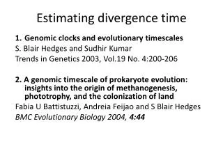
1. Estimating divergence time Genomic clocks and evolutionary timescales S. Blair Hedges and Sudhir Kumar Trends in Genetics 2003, Vol.19 No. 4:200-206 2. A genomic timescale of prokaryote evolution: insights into the origin of methanogenesis, phototrophy, and the colonization of land Fabia U Battistuzzi, Andreia Feijao and S Blair Hedges BMC Evolutionary Biology 2004, 4:44

2. Things you need to get a date 1. Organisms (interested) 2. A phylogram describes -the relationships -the number of evolutionary changes along a branch -the branch lengths represent nucleotide substitutions. 3. Black box of dating methods 4. External information on time -fossil records 5.Branch length + evolutionary rate + time (age) -- result to chronogram -the branch lengths represent time units between divergences

3. A genomic timescale of prokaryote evolution (Background) • The timescale of prokaryote evolution has been difficult to reconstruct. • 1. A limited fossil record • Some elements have forms (called isotopes) with unstable atomic nuclei that have a tendency to change, or decay. • U-235 (unstable isotope or parent isotope) • Pb-207(daughter isotope) • Where the amounts of parent and daughter isotopes can be accurately measured, the ratio can be used to determine how old the rock is. • For eukaryotes, the fossil record provides an abundant source of such data, but this has not been true for prokaryotes, which are difficult to identify as fossils • In 1999, the analysis of cyanobacteria-specific molecular fossil such as 2-methylhopanoid as biomarker s for cyanobacterial oxygenic photosynthesis have shown that late Archean shales dated to ages between 2.04 and 3.08 Ga and allowed calibration of distance trees and permits estimates of the major prokaryotic divergences.

4. A genomic timescale of prokaryote evolution (Background) • 2. complexities associated with molecular clocks and deep divergences. • Horizontal gene transfer (HGT) is any process in which an organism transfers genetic material to another cell that is not its offspring. This events are of great interest in their roles to create functionally new combinations of genes, but they pose problems for investigating the phylogenetic history and divergence times of organisms. • S. Garcia-Vallve, E. Guzman, MA. Montero and A. Romeu. 2003. HGT-DB: a database of putative horizontally transferred genes in prokaryotic complete genomes.Nucleic Acids Research 31(1):187-189

5. What is molecular clock? • The molecular clock is a technique in genetics to date when two species diverged. Elapsed time is deduced by applying a time scale to the number of molecular differences measures between the species' sequence or proteins • Current molecular clock methods are three basic approaches for analysis of multiple genes or protein; • 1. Methods that use a molecular clock and one global rate of substitution • 2. Methods that correct for rate heterogeneity or local clock • 3. Methodss that try to incorporate rate heterogeneity • There are two basic approaches to estimate divergence time when data from multiple constant-rate genes or rate heterogeneity; Multigene method and Supergene method

6. The difference of data sets • Multigene method • 1. divergence time are estimated for each gene separately • 2. the average or modal divergence time and error is estimated from pooled time estimates • 3. Multigene time distributions are usually symmetric and have a strong central tendency • 4.This method can be used with genes having widely varying species samples and rate of change • Supergene method • 1.concatenating nucleotide or protein sequences from all relevant genes of a species to form a single alignment for time estimation • 2. rate variation between genes and among sites within genes should be modeled • 3. evolutionary distance between species can be computed for each gene and then averaged over all genes for a given species pair. • 4.divergence time is estimated by dividing the average distance by the average calibration distance.

7. Global clock or one global rate of substitution method • all branches of a phylogenetic tree evolve at the same, global substitution rate. The clock-like tree is ultrametric, which means that the total distance between the root and every tip is constant • If a data set follows a clock, the evolutionary rate is constant over time, and the branch lengths equal the product of rate and time. • the branch lengths can be used to infer relative rates and times • Relative rate tests are used in almost all global clock studies. Genes and lineages that are rejected in the rate tests are usually removed from later analyses. Each gene that is not rejected in the relative rate tests can be considered to be evolving under a constant rate of substitution.

8. Table 1 Comparison table of different molecular dating methods.Part 1: Methods that use a molecular clock and one global rate of substitution §PAUP* (Swofford, 2001), DNAMLK(part of the PHYLIP package; Felsenstein, 1993), BASEML (part of the PAML package; Yang, 1997), MRBAYES(Huelsenbeck and Ronquist, 2001), BEAST(Drummond & Rambaut, 2003), etc Advantage - The global molecular clock seemed to be very useful for calculating divergence times and set up models of evolution for many group of organisms Drawback - the clock turned out to be an oversimplified model, and many studies presented highly unlikely results. Comparisons with the fossil record often showed large discrepancies between molecular and fossil ages

9. Local clock or heterogeneity rate of substitution method • Several reasons are given for these deviations from the clock-like model of sequence evolution; generation time, metabolic rate, mutation rate and population size • Local clock methods use a model of nucleotide or amino acid substitution in which rate is not constant among all branches by dividing the global rate into several rate classes (local rates). • Uses Bayesian inference methodology and maximum likelihood to estimate divergence time • Advantage-Local clock methods are promising as they can use genes discarded by global clock methods, permitting a larger total number of genes for estimating time, a positive attribute in data-limited situations. • Drawback-some assignments of rates to branches are not feasible as they cause the model to become unidentifiable.

10. Table 2 Comparison table of different molecular dating methods.Part 2: Methods that correct for rate heterogeneity

11. Methods that estimate divergence times byincorporating rate heterogeneity • Methods that relax rate constancy must necessarily be guided by specifications about how rates are expected to change among lineages • All methods estimate branch lengths without assuming rate constancy, and then model the distribution of divergence times and rates by minimizing the discrepancies between branch lengths and the rate changes over the branches. • The methods differ in their strategy to incorporate age constraints (calibration points) into the analysis.

12. Table 3 Comparison table of different molecular dating methods. Part 3: Methods that incorporate rate heterogeneity

13. Prokaryote evolution timescale • In 2004 , Battistuzzi et al has been reconstructed the genomic timescale of prokaryote from a data set of sequences currently available from 32 proteins common to 72 species. • They estimated phylogenetic relationships and divergence times with a local clock method. • Assembled many family protein and many species

14. The objective of this study • The most information on the timescale of prokaryote evolution has come from analysis of DNA and amino acid sequence data with molecular clocks. • The increasing number of prokaryotic genomes available has facilitated the detection of HGT through more accurate detection of orthology, paralogy, and monophyletic groups, and the concatenation of gene and protein sequences has helped increase the confidence of nodes and decrease the variance of time estimates. • 1. To assemble a data set of sequences from 32 proteins (~7600 amino acids) common to 72 species. • 2. To estimate phylogenetic relationships and divergence times with a local clock method. • 3. To investigate the origin of metabolic pathways of importance in evolution of the biosphere.

15. Methods(Data assembly) • Data assembly began with the Clusters of Orthologous Groups of Proteins (COG), is a systematic grouping of gene families that have completed genomes.  These groups are formulated by comparing protein sequences of known origin to those proteins of unicellular genomes which have been studied extensively, have a phylogenetic lineage, and have been deemed complete.  • A COG consists of a protein or  group of proteins typically paralogs that come from a minimum of 3 lineages which will ultimately correspond to an ancestral domain.   Currently 66 clusters exist and with more research and study the list will continue to expand. • In this study, COGs consisted of 84 proteins common to 43 species. • With that initial dataset, other species from among completed microbial genomes (NCBI; National Center for Biotechnology Information) assisted by BLAST and PSI-BLAST were added. • In total 72 species were included in the study (54 eubacteria, 15 archaebacteria and three eukaryotes were Arabidopsis thaliana, Drosophila melanogaster, and Homo sapiens). • This dataset consisted of 60 proteins that were individually analyzed as a step in orthology determination. • The proteins were aligned with CLUSTALW .

16. Methods(Data assembly) • Phylogenetic trees of each protein were built and visually inspected. Initial trees were constructed using Minimum Evolution (ME), with MEGA version 2.1. • Minimum Evolution method (ME) is the method that the expected value of the sum of all branch lengths (S) is smallest for the true tree or as the best tree. • S = T∑i bi ; • bi = estimate of the length of the i-th branch and T is the total number of branch 3.9 6.2 4.5 -2.1 -2.4 7.6 9.5 6.1 7.5 14.4 11.7 14.3 5.3 11.8 12.1 S = 37.6 S = 35.3 S = 37.5 Estimates of branch lengths obtained by ME

17. Methods(Data assembly) • The major criterion used in determining which genes to include or exclude was the monophyly of domains. • Monophyly taxon is a group of organisms descended from a single ancestor. Polyphyletic taxon is composed of unrelated organisms descended from more than one ancestor. One type of monophyletic taxon is a paraphyletic taxon, which includes an ancestor and a group of organisms descended from it.

18. Methods(Data assembly) • Rejected genes with domains (arcaebacteria and eubacteria) that were non-monophyletic, as these would be the best examples of HGT, this amounted to 61% of the genes rejected. • tested the effectiveness of the criteria by examining the stability of individual protein trees, using different gamma values (α = 1, 0.5 and 0.3).(???) • kept only the genes that were stable to such perturbations (in terms of remaining in that category of non-HGT genes). • The 32 remaining proteins were concatenated for analysis. The majority (81%) of the 32 proteins that were used are classified in the "information storage and processes" functional category of the COG. The other categories represented are "cellular processes" (10%), "metabolism“ (3%), and "information storage and processing" + "metabolism" (proteins with combined functions; 6%). • From the concatenation, trees were constructed with ME, Maximum Likelihood (ML)(log likelihood score, optimized over branch lengths and model parameter) and Bayesian methods (Posterior probability, calculated by integrating over branch lengths and substitution parameter).

19. Result (Phylogeny) • The phylogenies obtained with ME, ML and Bayesian were similar, differing only at nonsignificant nodes assessed by the bootstrap method. • Bootstrap test method is the method of testing the reliability of the topology of a tree obtained by distance methods. This test examine the reliability of each interior branch of a tree by computing the probability of confidence which is called bootstrap value. Nucleotide or amino acid sites are sampled randomly, with replacement, and new tree is constructed. This is repeated many times and the frequency of appearance of a particular node. If the value is higher than 95%, the interior branch is considered to be statistically significant. • The phylogeny of eubacteria (Fig. 1) shows significant bootstrap support for most of the major groups and subgroups. • 1.All proteobacteria form a monophyletic group (support values 95/47/99 for ME, ML and Bayesian respectively) with the following relationships of the subgroups: (epsilon (alpha (beta, gamma))).

20. Result(Phylogeny) • 2.There has been debate about the effect of base composition and substitution rate on the phylogenetic position of the endosymbiont Buchnera among γ-proteobacteria. Its position differs slightly from both studies; accordingly,any conclusions concerning its divergence time should be treated with caution. • 3.Spirochaetes cluster with Chlamydiae, Actinobacteria with Cyanobacteria and Deinococcus (support values for Cyanobacteria + Deinococcus are 92/80/99) and the hyperthermophiles (Thermotoga, Aquifex) branch basally in the tree. These groups and relationships are similar to those found previously with analyses of prokaryote genome sequences.

21. Figure1. Phylogenetic tree (ME; α = 0.94) of eubacteria rooted with archaebacteria, using sequences of 32 proteins (7,597 amino acids).Bootstrap values are shown on nodes; asterisks indicate support values > 95%. For major groups, support values from threephylogenetic methods (ME/ML/Bayesian) are indicated in italics (dash indicates a group was not present). 2 1 3

22. Result(Phylogeny) • 4.The phylogeny of archaebacteria (Fig. 2) agrees with some but not all aspects of previous phylogenetic analyses of prokaryote genomes using sequence data and the presence and absence of genes • For example, each of the two major clades of Archaebacteria is monophyletic. This is consistent with some analyses but not others. Also, the position of Crenarchaeota as closest relatives of eukaryotes (Fig. 2), instead of Euryarchaeota, has been debated. • 5.Methanogens were found to be monophyletic in some previous analyses but were paraphyletic in other analyses and in our analysis (Fig. 2). The phylogenetic position of one species of methanogen in particular, Methanopyrus kandleri, has differed among previous studies. However, it is difficult to make direct comparisons among various studies because they have included different sets of taxa.

23. Figure 2 Phylogenetic tree (ME; α = 1.20) of archaebacteria rooted with eubacteria, using sequences of 32 proteins (7,338 amino acids) Phylogenetic tree (ME; α = 1.20) of archaebacteria rooted with eubacteria, using sequences of 32 proteins (7,338 amino acids). Bootstrap values are shown on nodes; asterisks indicate support values > 95%. For major groups, support values from three phylogenetic methods (ME/ML/Bayesian) are indicated in italics. 5 4

24. Method (Time estimation) • Time estimation was conducted separately within each domain (Archaebacteria and Eubacteria) using reciprocal rooting and several calibration points. • All time estimates were calculated with a Bayesian local clock approach utilizing concatenated data sets of multiple proteins and a JTT+gamma model of substitution. • Bayesian local clock idea is that If evolutionary events (e.g.,nucleotide substitutions) occur independently, then the number of evolutionary events that occur on a branch existing from time 0 to time T and having rate R(t) at time t follows a Poisson distribution with mean • B(T) refer as a branch length. R(t) cannot be directly observed. One way to overcome this problem is to adopt the restrictive molecular clock assumption of a constant rate with respect to time. - The rate of branch i will be denoted Ri. The autocorrelation of rates between an ancestral branch and its direct descendant will depend on the time difference between the midpoints of the ancestral and the descendant branches. For example, the time difference between the thickened ancestral and descendant branches in figure 1 is

25. Method (Time estimation) • In Bayesian analyses, a priori knowledge about parameter values is summarized through assignment of probability distributions known as priors. • The observed data and the prior distributions are then used to determine probability distributions known as posteriors. • The posterior distribution is a probability distribution representing uncertainty about the parameters after observing the data. • The logarithm of the rate on the descendant branch has a normal distribution with a mean equal to the logarithm of the rate on the ancestral branch and with a variance equal to the time difference multiplied by a constant that we will refer to as v. A high value of v means there is little rate autocorrelation, and a low value implies strong rate autocorrelation. • By Bayesian convention, a parameter governing a prior distribution is called a hyperparameter. In this model, the value of v determines the prior distribution for the rates of molecular evolution on different branches given the internal node times. • Posterior Distribution, for a data set X of aligned homologous sequences, the posterior distribution depends on p(T, R, v | X) through • if both the rates R and the divergence times T are known, about the data X. Letting B = (B0, . . . , Bk) represent the lengths of the branches on the tree, we have The distribution p(T, R, v | X) is • because p(X |T, R) = p(X I B).

26. Method (Time estimation) • Calibration of rate in this method was implemented by assigning constraints to nodes in the phylogeny. Five different initial settings (prior distributions) were used in each domain. • These were chosen at intervals of 0.5 Ga starting from 4.5 Ga, which is approximately the age of the Earth and Solar System, to 2.5 Ga, which is slightly before the major rise in oxygen (Great Oxidation Event; GOE) as recorded in the geologic record and related to the presence of oxygenic cyanobacteria. • Those constraints pertained to the ingroup root, or deepest divergence in the tree excluding the outgroup. Because of the relatively small number of duplicate genes available for rooting the tree of life, we were unable to estimate the time of the last common ancestor (the divergence of eubacteria and archaebacteria).

27. Prior distribution for the rate of molecular evolution • sss -my understand is 2500, 3000, 3500, 4000 and 4500 Ma are the Calibration point as the time or age and we have branch length of data set from phylogram. So these two parameter will find out what is the rate (Rtrate) in each calibration time.

28. Chronogram of Archaebacteria

29. Time estimation * * The fossil calibration was the first appearance of a representative of the plant lineage (red algae) at 1.198 ± 0.022 Ga. The molecular time estimate for this divergence was 1.609 ± 0.060 Ga from a study of 143 rate-constant proteins.

30. Figure3. A timescale of prokaryote evolution * 100 * 29

31. Chronogram of Eubacteria

32. Time estimation * *

33. Time estimation • For the eubacterial data set, we used four internal time constraints in separate analyses, all involving the origin of cyanobacteria. • The first and most conservative constraint was a fixed origin (minimum and maximum bounds) at 2.3 Ga, which corresponds to the GOE. • For the second constraint we used 2.3 Ga as a minimum bound, with no maximum bound. • For the third constraint we used a previous molecular time estimate (2.56 Ga) for the divergence of cyanobacteria from closest living relatives among eubacteria, and fixed the minimum (2.04 Ga) and maximum (3.08 Ga) values to the 95% confidence limits of that time estimate. • The fourth constraint for the origin of cyanobacteria was set at 2.7 Ga (minimum constraint) based on biomarker evidence for the presence of 2α-methylhopanes . • The use of these four alternative constraints for the origin of cyanobacteria considers most of the widely discussed hypotheses but does not rule out an origin prior to 2.7 Ga. Although the results of the four different calibrations are provided for comparison, our preferred calibration is the 2.3 (minimum) geologic calibration because it has the best justification (supporting evidence).

34. Result (time estimation) • A single timetree was constructed from the phylogenetic and divergence time data. The time estimates summarized in that tree derive only from the best-justified calibrations. • For eubacteria, the 2.3 Ga minimum calibration (constraint), from the geologic record, was chosen because it encompasses all of the hypothesized time estimates for the origin of cyanobacteria. • For archaebacteria, the 1.2 Ga calibration (minimum 1.174 Ga, maximum 1.222 Ga), from the red algae fossil record, was selected because it provides a conservative constraint on the divergence of plants and animals.

35. 2. Discussion 8. 1.Hyperthermophiles • Most in basal Position • Debate in this tree 2. E.Coli and Salmonella is consistent. 3. Inconsistent with the fossil record that represented Cyanobacteria 4. Closely spaced in time of archaebacteria 9. 11. 10. 3. 1. 7. 6.. 4. 5.

36. Discussion 5. Origin of life on Earth • A Hadean (4.5–4.0 Ga) origin for life on Earth is also consistent with the early establishment of a hydrosphere. Nevertheless, the earliest geologic and fossil evidence for life has been debated leaving no direct support for such old time estimates. 6. Methanogenesis • Archaebacteria are the only prokaryotes known to produce methane. Our time estimate of between 4.11 Ga (3.31–4.49 Ga) (node P-O) and 3.78 Ga (3.05–4.16 Ga) for the origin of methanogenesis suggests that methanogens were present on Earth during the Archean, consistent with the methane greenhouse theory. 7. Anaerobic methanotrophy • Anaerobic methanotrophy, or anaerobic oxidation of methane (AOM), is a metabolism associated with oxidation of methane and sulfate reduction. The methane oxidizers are represented by archaebacteria phylogenetically related to the Methanosarcinales(at 3.09 (2.47–3.51) Ga ,node M to 0.23 Ga (0.12–0.39 Ga, node L), while the sulfate reducers, when present, are eubacterial members of the δ-proteobacteria division

37. Discussion 8. Aerobic methanotrophy • Both anaerobic and aerobic methanotrophy have been used to explain the highly depleted carbon isotopic values found in 2.8–2.6 Ga geologic formations. Divisions of the proteobacteria has been suggested an origin of this metabolism between (node C (2.80 Ga; 2.45–3.22 Ga) and node B (2.51 Ga; 2.15–2.93 Ga) ).The time estimates for these two metabolisms are both compatible with the isotopic record. 9. Phototrophy • The ability to utilize light as an energy source (phototrophy,photosynthesis) is restricted to eubacteria among prokaryotes. Phototrophic eubacteria are found in five major phyla (groups), including proteobacteria, green sulfur bacteria, green filamentous bacteria, gram positive heliobacteria, and cyanobacteria. This broad taxonomic distribution of phototrophic metabolism mechanism is HGT. They have assumed that the common ancestor (Node I) was phototrophic .Therefore, phototrophy evolved prior to 3.19 (2.80–3.63) Ga (node I). Because the hyperthermophiles Aquifex and Thermotoga are not phototrophic and branch more basally, 3.64 (3.17–4.13) Ga (Node J) can be considered a maximum date for phototrophy.

38. Discussion 10. The colonization of land • The synthesis of pigments such as carotenoids, which function as photoprotective compounds against the reactive oxygen species created by UV radiation, is an ability present in all the photosynthetic eubacteria and in groups that are partly or mostly associated with terrestrial habitats such as the actinobacteria, cyanobacteria, and Deinococcus-Thermus. Pigmentation was probably a fundamental step in the colonization of surface environments. An early colonization of land is inferred to have occurred after the divergence of this terrestrial lineage with Firmicutes (node H), 3.05 (2.70–3.49) Ga, and prior to the divergence of Actinobacteria with Cyanobacteria + Deinococcus (node F), 2.78 (2.49–3.20) Ga. These molecular time estimates are compatible with time estimates (2.6–2.7 Ga) based on geological evidence for the earliest colonization of land by organisms (prokaryotes). 11. Oxygenic photosynthesis • some of the early steps leading to oxygenic photosynthesis apparently were acquisition of protective pigments, phototrophy, and the colonization of land. Species of cyanobacteria are known, broadly distributed among the orders. The origin of cyanobacteria as a calibration was 2.3 Ga, geologic time based on GOE. In this case, the time estimated for node E (2.56 Ga; 2.31–2.97 Ga) was not much older than the constraint itself

39. Figure 4 A time line of metabolic innovations and events on EarthA time line of metabolic innovations and events on Earth. The minimum time for oxygenic photosynthesis is constrained by the Great Oxidation Event (2.3 Ga) whereas the maximum time for the origin of life is constrained by the origin of Earth (4.5 Ga). Horizontal lines indicate credibility intervals, white boxes indicate minimum and maximum time constraints on the origin of a metabolism or event, and colored boxes indicate the presence of the metabolism or event.

40. Our phylogenetic results support most of the currently recognized higher-level groupings of prokaryotes. Divergence time estimates for the major groups of eubacteria are between 2.5–3.2 billion years ago (Ga) while those for archaebacteria are mostly between 3.1–4.1 Ga. The time estimates suggest a Hadean origin of life (prior to 4.1 Ga), an early origin of methanogenesis (3.8–4.1 Ga), an origin of anaerobic methanotrophy after 3.1 Ga, an origin of phototrophy prior to 3.2 Ga, an early colonization of land 2.8–3.1 Ga, and an origin of aerobic methanotrophy 2.5–2.8 Ga. Conclusions: Our early time estimates for methanogenesis support the consideration of methane, in addition to carbon dioxide, as a greenhouse gas responsible for the early warming of the Earths‘ surface. Our divergence times for the origin of anaerobic methanotrophy are compatible with highly depleted carbon isotopic values found in rocks dated 2.8–2.6 Ga. An early origin of phototrophy is consistent with the earliest bacterial mats and structures identified as stromatolites, but a 2.6 Ga origin of cyanobacteria suggests that those Archean structures, if biologically produced, were made by anoxygenic photosynthesizers. The resistance to desiccation of Terrabacteria and their elaboration of photoprotective compounds suggests that the common ancestor of this group inhabited land. If true, then oxygenic photosynthesis may owe its origin to terrestrial adaptations.