Expected Present value - project A

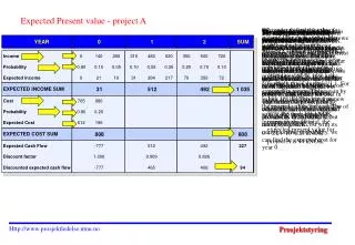
1. YEAR 0 1 2 SUM Income 0 140 200 310 480 620 350 500 720 Probability 0.80 0.15 0.05 0.10 0.55 0.35 0.20 0.70 0.10 Expected income 0 21 10 31 264 217 70 350 72 EXPECTED INCOME SUM 31 512 492 1 035 Cost 765 980 Probability 0.80 0.20 Expected Cost 612 196 EXPECTED COST SUM 808 808 Expected Cash Flow -777 512 492 227 Discount factor 1.000 0.909 0.826 Discounted expected cash flow -777 465 406 94 We repeat this step for the income amount in year 0. Here we have three possible outcomes: 0, 140 and 200 kNOK. These values are multiplied with their respective probabilities: 80%, 15% and 5%, which gives us three expected incomes. These values are independent from the progress of the project. The sum of the three expected incomes in year 0 is: 0 + 21 + 10 = 31 kNOK In order to find the value for capital for each of the years, we will use a discount factor corresponding to a 10% interest rate. We find this value in year 0, where it is equal to the starting value. In year 1, we multiply this value by 1/1,1. For year two, we multiply again by 1/(1,1*1,1). This gives us new expected values for cashflow of 777, 465 and 406 kNOK respectively. In total, the expected present value for project A is 94 kNOK. The corresponding probabilities for these values are shown as well. Expected Present value - project A The costs for the entire the 3-year period is 808000 NOK, with costs occuring only in year 0. The expected income for the three-year period is: 31 + 512 + 492 = 1035 kNOK When we have expected incomes and expected costs, we can find the expected cash flow by subtracting the expected cost from the expected income. The expected value concept says that we calculate the expected values and use them as the decision basis. Therefore, we will use the expected cost value of 808 kNOK as the decision basis. By adding 612 kNOK and 196 kNOK, we get a value of 808 kNOK for expected cost. This value is not a real value for our project, but if we implement the project many times, the average value of the costs for year 0 becomes 808000 NOK. Once we implement the project, the cost of the investment will be 765 kNOK or 980 kNOK, but never 808 kNOK. In year 0, the project will have an investment of 765000 NOK. Little uncertainty is connected to this investment. It is 20% likely that the project will have cost-overrun, which means costs in year 0 could become 980000 NOK. Because we have two possible magnitudes for cost in year 0, there are two possible outcomes that form a discrete probability distribution. By multiplying each cost with its corresponding probability, we can find the expected cost for year 0. For each year, income and cost values are set up in the table. We will choose one of two projects, A or B. Project A, shown on the left side of table, happens over a 3-year period from year 0 to year 2. We will repeat this step for year 1. Three different incomes with corresponding probabilities give us three expected incomes. Altogether, this gives us 512 kNOK in year 1. The income for year 1 never equals 512 kNOK, but either 31,264 or 217 kNOK. The same is done for year 2, where the sum of the expected incomes is 492 kNOK. Http://www.prosjektledelse.ntnu.no

2. PRESENT VALUE PROBABILITY EXPECTED VALUE 30 0.10 3 50 0.30 15 80 0.35 28 100 0.25 25 SUM 71 Expected Present value - project B In project B, there are four outcomes for present value and its corresponding probability. We can now use the usual procedure to find the expected value. Once we have calculated for each outcome and add them together, we get an end sum of 71 kNOK. Outcome 1 has a present value of 30 kNOK and a probability of 10%. This gives us an expected value of 3 kNOK Http://www.prosjektledelse.ntnu.no

3. Project A 94 Project B 71 We can now see that project A has the highest expected present value and therefore should be preferred to project B. Both projects have values that do not happen in reality. The amounts that we have calculated only serve for the purpose of comparing the two projects. Http://www.prosjektledelse.ntnu.no