Download

1 / 53
540 likes | 875 Views
Receptor Modeling Source Apportionment for Air Quality Management. John G. Watson (john.watson@dri.edu) Judith C. Chow Desert Research Institute Reno, Nevada, USA. Presented at: The Workshop on Air Quality Management, Measurement, Modeling, and Health Effects

E N D
Receptor Modeling Source Apportionment for Air Quality Management John G. Watson (john.watson@dri.edu) Judith C. Chow Desert Research InstituteReno, Nevada, USA Presented at:The Workshop on Air Quality Management, Measurement, Modeling, and Health Effects University of Zagreb, Zagreb, Croatia 24 May 2007
Objectives • Review receptor models and data requirements • Summarize prior uses of receptor models in air quality management • Describe strategies for separating primary and secondary source contributions
Black Carbon (BC) Remains at Mesa Verde National Park, Colorado, USA • Not all BC is from diesel and other vehicular emissions • “Marker” is a better term than “tracer” • There’s something of everything in everything
Source and Receptor Models The source model uses source emissions as inputs and calculates ambient concentrations. The receptor model uses ambient concentrations as inputs and calculates source contributions. (From Watson, 1979.)
Cikl = ΣjΣmΣn TijklmnDklnFijQjkmn CALCULATED BY CHEMICAL MODEL CALCULATED AT RECEPTOR CALCULATED BY MET MODEL MEASURED AT SOURCE (INVENTORY) Lagrangian Source Model CMB Receptor Model Cikl = ΣjTijklFijΣmΣn DklnQjkmn MEASURED AT RECEPTOR MEASURED AT SOURCE (T=1 OR ESTIMATED BY OTHER METHOD Sijkl, SOURCE CONTRIBUTION ESTIMATE
Chemical Mass Balance • Equation: • Input: • Ambient concentrations (Ci)and uncertainties (sCj),source profiles (Fij),and uncertainties (sFij). • Output: • Source contributions (Sj)and uncertainties (sSj). • Measurements: • Size-classified mass, elements, ions, and carbon concentrations on both ambient and source samples.
CMB SolutionsMinimize differences between calculated and measured values for overdetermined set of equations ϰ2 = minΣi [(Ci-Ci)2/ϭCi2] + ΣiΣi[(Fij-Fij)2/ϭFij2] Britt and Luecke, (1973), single sample, bold=true value ϰ2 =minΣi[(Ci-ΣjFijSj)2/(ϭCi2+ΣjϭFij2Sj2)] Effective Variance, Watson et al., (1984), single sample ϰ2 =minΣi[(Ci-ΣjFijSj)2/ϭCi2)] Ordinary Weighted Least Squares, Friedlander (1973), single sample
Other CMB Solutions Sj=Ci/Fij Tracer solution, Hidy and Friedlander (1971), Winchester and Nifong (1971), single sample ϰ2 =minΣk[(Massk-ΣiCik/Fii)2] Multiple Linear Regression, Kleinman et al (1980), multiple samples ϰ2 =minΣiΣk[(Cik-ΣjFijSjk)2/ϭCik2)] Positive Matrix Factorization, Paatero (1997), multiple samples
Receptor Models are Not Statistical • They don’t test hypotheses or determine statistical significance • Receptor models should be physically based with statements of simplifying assumptions and evaluation of deviations from assumptions • They infer mechanisms and interactions rather than explicitly calculate them • Receptor models recognize and elucidate patterns in measured components, space and time that bound the types, quantities, and locations of source contributions • Some of them explicitly use input data uncertainties to weight influence of inputs and estimate uncertainties of outputs
Types of “Modern” Receptor Models • Chemical Mass Balance CMB with various solutions including marker (trace method, effective variance (EV), principal component analysis (PCA), UNMIX, abd positive matrix factorization (PMF) solutions • Aerosol Evolution and Equilibrium Estimates how reduction in one precursor will affect PM end-products • Back Trajectory estimates source areas for different pollutants or source contributions
Chemical Mass Balance • Equation: • Input: • Ambient concentrations (Ci)and uncertainties (sCj),source profiles (Fij),and uncertainties (sFij). • Output: • Source contributions (Sj)and uncertainties (sSj). • Measurements: • Size-classified mass, elements, ions, and carbon concentrations on both ambient and source samples.
Receptor Measurements from Ambient Samplers Airmetrics portable MiniVol sampler BGI FRM Omni PM1, PM2.5, and PM10 PM2.5 and PM10
Many contributors not inventoried Real-World Cooking Simulated Cooking
More source profiles could be obtained from certification tests Roadside compliance test in India
Material balance says much about sources(Mexico City, Feb/Mar 1997) (Chow et al., 2002)
More specificity obtained with source profiles Commonly measured elements, ions, and carbon (Zielinska et al., 1998)
Many toxic elements have been removed from emissions.Organic markers take their place (Chow et al. 2006)
Carbon fractions have been found useful and can be obtained from existing samples (Watson et al., 1994) Gasoline-fueled vehicles Diesel-fueled vehicles
Thermally-evolved material can be separated by chromatography and mass spectrometryChallenge is to extract information that separates sources Gasoline Coal power plant Diesel Roadside dust
Examples of U.S. CMB Model Air Quality Findings and Results • Oregon wood stove emissions standard (Watson, 1979) • Midwest contributions to east coast sulfate and ozone (Wolff et al., 1977, Lioy et al., 1980, Mueller et al., 1983, Rahn and Lowenthal, 1984) • Washoe County, Nevada, stove changeout, burning ban, and “squealer” number (Chow et al., 1989) • California EMFAC emissions model revisions (Fujita et al., 1992, 1994) • SCAQMD (Los Angeles) grilling emission standard (Rogge, 1993) • SCAQMD (Los Angeles) street sweeper specification (Chow et al., 1990)
Examples of U.S. CMB Model Air Quality Findings and Results (continued) • SCAQMD (Los Angeles) Chino dairy reduction (NH3) regulation (SCAQMD, 1996) • PM10 SIP implementation of wood burning, road dust, and industrial emission reductions (Davis and Maughan, 1984, Houck et al., 1981, 1982, Cooper et al., 1988, 1989) • Navajo Generating Station SO2 scrubbers (Malm et al., 1989) • Hayden Generating Station SO2 scrubbers (Watson et al., 1996) • Mohave Generating Station shutdown (Pitchford et al., 1999) • Denver Colorado urban visibility standard (Watson et al., 1988)
Worldwide PM Source Contribution Estimates by Chemical Mass Balance(Chow and Watson, 2002)
Receptor Model Results Need to be ChallengedCMB Sensitivity Test (Chow et al. 2006)
CMB Pseudo-Inverse Normalized (MPIN) Matrix (Chow et al. 2006)
One Atmosphere (Gases and Particles) Also Works for Receptor Models (Gertler et al., 1996) Light Duty Emission Rates Heavy Duty Emission Rates
Hourly (VOC) data provide temporal corroboration of emissions and reveal unknown sources(Houston, TX, 1993) (Lu, 1996) Unknown event Morning traffic
High Time Resolution is DesiredSpikes indicate local sources (Watson and Chow, 2001)
Wind Direction is Suggestive for Local Sources Conditional Probability Function (CPF) for a Selenium Factor at the Pittsburg Supersite (Pekney et al., 2006)
Source factors derived from ambient data by UNMIX and PMFThese must be associated with measured source profiles(Chen et al., 2006)
Markers for Biogenic SOA(Pandis, 2001) • Pinic acid, pinonic acid, norpinic acid, and norpinonic acid are products of the oxidation of most monoterpenes • There are some (apparently) unique tracers: • Hydropinonaldehydes for α-pinene • Nopinone for β-pinene • 3-caric acid for carene • Sabinic acid for sabenene • Several of these compounds measured in field studies in forests (usually a few nanograms per cubic meter, sometimes as much as 0.1 µg m-3)
SO4=/SO2 Ratio changes during Aerosol Aging (and should be Reflected in Source Profiles) (Watson et al., 2002)
Back trajectories indicate source regions (Xu et al., 2006) Regression parameters for Grand Canyon National Park (2000–2002). Percent of time the parcel is in a horizontal grid cell based on back trajectories starting at 500 m.
Receptor Models Can Estimate the Future in Some Circumstances(Denver, CO, 1997) (Watson et al., 1998) Effect of ammonia reductions on ammonium nitrate particles Effect of nitric acid reductions on ammonium nitrate particles
Emission Reduction EffectivenessLong-Term Trends in SO2 Emissions and SO4= Levels(Malm et al., 2002)
Murphy’s Law of Reproducibility“If reproducibility is a problem, just use one model”Mohave Generating Station contributions to Meadview sulfate (Pitchford et al., 1999)
Model discrepancies help to improve inventoriesPM2.5 Inventory/Receptor Model Comparison, Denver, CO (1997)(Watson et al., 2002)
SIP Guidance “Weight of Evidence” Approach(EPA, 2001) • Form a conceptual model of the emissions, meteorology, and chemical transformations that are likely to affect exceedances • Develop a modeling/data analysis protocol with stakeholders consistent with available science, measurements, and the conceptual model • Construct and evaluate emission inventory for the domain as indicated by the conceptual model
SIP Guidance “Weight of Evidence” Approach(continued) • Assemble and evaluate meteorological measurements for the domain • Apply source and receptor models and to determine contributions • Apply diagnostic tests and justify discarding results that are not physically reasonable
SIP Guidance “Weight of Evidence” Approach(continued) • Modify the inventory to reflect different emission reduction strategies in consultation with stakeholders, and evaluate the effects of reductions at receptors • Make models, input data, and results available to others for external review • Judge the weight of evidence supporting or opposing the selected emission reduction strategy prior to implementation
Receptor Model Needs: A Summary • Source properties that identify and quantify source contributions at a receptor (Daisey et al., 1986, Gordon et al., 1984) • Better designed networks (Chow et al., 2002, Demerjian, 2000) with respect to • Sampling locations • Sampling periods • Sample durations • Particle sizes • Precursor gases • Chemical and physical components • Meteorology
Receptor Model Needs(continued) • Emissions profiles (with cooling and dilution including marker species and gases, (England et al., 2000) • More convenient availability and documentation of source profile and ambient data (U.S. EPA, 1999) • More evaluation, validation, and reconciliation of receptor and source modeling results (Javitz et al., 1988)
References Cabada, J.C.; Pandis, S.N.; and Robinson, A.L. (2002). Sources of atmospheric carbonaceous particulate matter in Pittsburgh, Pennsylvania. J. Air Waste Manage. Assoc., 52(6):732-741. Cabada, J.C.; Pandis, S.N.; Subramanian, R.; Robinson, A.L.; Polidori, A.; and Turpin, B.J. (2004). Estimating the secondary organic aerosol contribution to PM2.5 using the EC tracer method. Aerosol Sci. Technol., 38(Suppl. 1):140-155. ISI:000221762100013. Chen, L.-W.A.; Chow, J.C.; Watson, J.G.; Lowenthal, D.H.; and Chang, M.C. (2006). Quantifying PM2.5 source contributions for the San Joaquin Valley with multivariate receptor models. Environ. Sci. Technol., submitted. Chow, J.C.; Engelbrecht, J.P.; Watson, J.G.; Wilson, W.E.; Frank, N.H.; and Zhu, T. (2002a). Designing monitoring networks to represent outdoor human exposure. Chemosphere, 49(9):961-978. ISI:000179483700007. Chow, J.C.; and Watson, J.G. (2002). Review of PM2.5 and PM10 apportionment for fossil fuel combustion and other sources by the chemical mass balance receptor model. Energy & Fuels, 16(2):222-260. http://pubs3.acs.org/acs/journals/doilookup?in_doi=10.1021/ef0101715. Chow, J.C.; Watson, J.G.; Edgerton, S.A.; Vega, E.; and Ortiz, E. (2002b). Spatial differences in outdoor PM10 mass and aerosol composition in Mexico City. J. Air Waste Manage. Assoc., 52(4):423-434. Chow, J.C.; Watson, J.G.; Egami, R.T.; Frazier, C.A.; and Lu, Z. (1989). The State of Nevada Air Pollution Study (SNAPS): Executive summary. Report No. DRI 8086.5E. Prepared for State of Nevada, Carson city, NV, by Desert Research Institute, Reno, NV. Chow, J.C.; Watson, J.G.; Egami, R.T.; Frazier, C.A.; Lu, Z.; Goodrich, A.; and Bird, A. (1990). Evaluation of regenerative-air vacuum street sweeping on geological contributions to PM10. J. Air Waste Manage. Assoc., 40(8):1134-1142. Chow, J.C.; Watson, J.G.; Lowenthal, D.H.; Chen, L.-W.A.; Zielinska, B.; Rinehart, L.R.; and Magliano, K.L. (2006). Evaluation of organic markers for chemical mass balance source apportionment at the Fresno Supersite. Chemosphere, submitted. Cooper, J.A.; Miller, E.A.; Redline, D.C.; Spidell, R.L.; Caldwell, L.M.; Sarver, R.H.; and Tansyy, B.L. (1989). PM10 source apportionment of Utah Valley winter episodes before, during, and after closure of the West Orem steel plant. Prepared for Kimball, Parr, Crockett and Waddops, Salt Lake City, UT, by NEA, Inc., Beaverton, OR.
References Cooper, J.A.; Sherman, J.R.; Miller, E.; Redline, D.; Valdonovinos, L.; and Pollard, W.L. (1988). CMB source apportionment of PM10 downwind of an oil-fired power plant in Chula Vista, California. In Transactions, PM10: Implementation of Standards, C.V. Mathai and D.H. Stonefield, Eds. Air and Waste Management Association, Pittsburgh, PA, pp. 495-507. Daisey, J.M.; Cheney, J.L.; and Lioy, P.J. (1986). Profiles of organic particulate emissions from air pollution sources: Status and needs for receptor source apportionment modeling. J. Air Poll. Control Assoc., 36(1):17-33. Davis, B.L.; and Maughan, A.D. (1984). Observation of heavy metal compounds in suspended particulate matter at East Helena, Montana. J. Air Poll. Control Assoc., 34(12):1198-1202. Demerjian, K.L. (2000). A review of national monitoring networks in North America. Atmos. Environ., 34(12-14):1861-1884. Eatough, D.J.; Du, A.; Joseph, J.M.; Caka, F.M.; Sun, B.; Lewis, L.; Mangelson, N.F.; Eatough, M.; Rees, L.B.; Eatough, N.L.; Farber, R.J.; and Watson, J.G. (1997). Regional source profiles of sources of SOX at the Grand Canyon during Project MOHAVE. J. Air Waste Manage. Assoc., 47(2):101-118. England, G.C.; Zielinska, B.; Loos, K.; Crane, I.; and Ritter, K. (2000). Characterizing PM2.5 emission profiles for stationary sources: Comparison of traditional and dilution sampling techniques. Fuel Processing Technology, 65:177-188. Forrest, J.; and Newmann, L. (1973). Sampling and analysis of atmospheric sulfur compounds for isotope ratio studies. Atmos. Environ., 7(5):561-573. Fujita, E.M.; Croes, B.E.; Bennett, C.L.; Lawson, D.R.; Lurmann, F.W.; and Main, H.H. (1992). Comparison of emission inventory and ambient concentration ratios of CO, NMOG, and NOx in California's South Coast Air Basin. J. Air Waste Manage. Assoc., 42(3):264-276. Fujita, E.M.; Watson, J.G.; Chow, J.C.; and Lu, Z. (1994). Validation of the chemical mass balance receptor model applied to hydrocarbon source apportionment in the Southern California Air Quality Study. Enivron. Sci. Technol., 28(9):1633-1649. Gertler, A.W.; Fujita, E.M.; Pierson, W.R.; and Wittorff, D.N. (1996). Apportionment of NMHC tailpipe vs non-tailpipe emissions in the Fort McHenry and Tuscarora mountain tunnels. Atmos. Environ., 30(12):2297-2305.
References Gordon, G.E.(1984). Atmospheric tracers of opportunity from important classes of air pollution sources. In DOE Workshop on Atmospheric Tracers, Santa Fe, NM. Gray, H.A.; Cass, G.R.; Huntzicker, J.J.; Heyerdahl, E.K.; and Rau, J.A. (1986). Characteristics of atmospheric organic and elemental carbon particle concentrations in Los Angeles. Enivron. Sci. Technol., 20(6):580-589. Hidy, G.M. (1987). Conceptual design of a massive aerometric tracer experiment (MATEX). J. Air Poll. Control Assoc., 37(10):1137-1157. Houck, J.E.; Cooper, J.A.; Core, J.E.; Frazier, C.A.; and deCesar, R.T. (1981). Hamilton Road Dust Study: Particulate source apportionment analysis using the chemical mass balance receptor model. Prepared for Concord Scientific Corporation, by NEA Laboratories, Inc., Beaverton, OR. Houck, J.E.; Cooper, J.A.; Frazier, C.A.; and deCesar, R.T. (1982). East Helena Source Apportionment Study: Particulate source apportionment analysis using the chemical mass balance receptor model, Vol. III Appendices. Prepared for State of Montana, Dept. of Health & Environmental Sciences, Helena, MT, by NEA Laboratories, Inc., Beaverton, OR. Javitz, H.S.; Watson, J.G.; Guertin, J.P.; and Mueller, P.K. (1988). Results of a receptor modeling feasibility study. J. Air Poll. Control Assoc., 38(5):661-667. Lewis, C.W.; and Stevens, R.K. (1985). Hybrid receptor model for secondary sulfate from an SO2 point source. Atmos. Environ., 19(6):917-924. Lioy, P.J.; Samson, P.J.; Tanner, R.L.; Leaderer, B.P.; Minnich, T.; and Lyons, W.A. (1980). The distribution and transport of sulfate "species" in the New York area during the 1977 Summer Aerosol Study. Atmos. Environ., 14:1391-1407. Lu, Z. (1996). Temporal and spatial analysis of VOC source contributions for Southeast Texas. Ph.D Dissertation, University of Nevada, Reno. Malm, W.C.; Pitchford, M.L.; and Iyer, H.K. (1989). Design and implementation of the Winter Haze Intensive Tracer Experiment - WHITEX. In Transactions, Receptor Models in Air Resources Management, J.G. Watson, Ed. Air & Waste Management Association, Pittsburgh, PA, pp. 432-458. Malm, W.C.; Schichtel, B.A.; Ames, R.B.; and Gebhart, K.A. (2002). A ten-year spatial and temporal trend of sulfate across the United States. J. Geophys. Res., 107(D22):ACH 11-1-ACH 11-20.