Download
1 / 34
350 likes | 502 Views
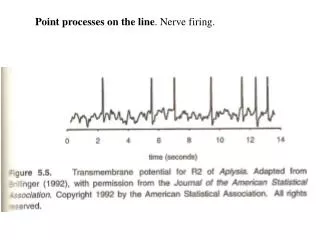
Point processes on the line . Nerve firing. Stochastic point process . Building blocks Process on R {N(t)}, t in R, with consistent set of distributions Pr{N(I 1 )=k 1 ,..., N(I n )=k n } k 1 ,...,k n integers 0 I's Borel sets of R.

E N D
Stochastic point process. Building blocks Process on R {N(t)}, t in R, with consistent set of distributions Pr{N(I1)=k1 ,..., N(In)=kn } k1 ,...,kn integers 0 I's Borel sets of R. Consistentency example. If I1 , I2 disjoint Pr{N(I1)= k1 , N(I2)=k2 , N(I1 or I2)=k3 } =1 if k1 + k2 =k3 = 0 otherwise Guttorp book, Chapter 5
Points: ... -1 0 1 ... discontinuities of {N} N(t) = #{0 < j t} Simple: j k if j k points are isolated dN(t) = 0 or 1 Surprise. A simple point process is determined by its void probabilities Pr{N(I) = 0} I compact
Conditional intensity. Simple case History Ht = {j t} Pr{dN(t)=1 | Ht } = (t:)dt r.v. Has all the information Probability points in [0,T) are t1 ,...,tN Pr{dN(t1)=1,..., dN(tN)=1} = (t1)...(tN)exp{- (t)dt}dt1 ... dtN [1-(h)h][1-(2h)h] ... (t1)(t2) ...
Parameters. Suppose points are isolated dN(t) = 1 if point in (t,t+dt] = 0 otherwise 1. (Mean) rate/intensity. E{dN(t)} = pN(t)dt = Pr{dN(t) = 1} j g(j) = g(s)dN(s) E{j g(j)} = g(s)pN(s)ds Trend: pN(t) = exp{+t} Cycle: cos(t+)
Product density of order 2. Pr{dN(s)=1 and dN(t)=1} = E{dN(s)dN(t)} = [(s-t)pN(t) + pNN (s,t)]dsdt Factorial moment
Autointensity. Pr{dN(t)=1|dN(s)=1} = (pNN (s,t)/pN (s))dt s t = hNN(s,t)dt = pN (t)dt if increments uncorrelated
Covariance density/cumulant density of order 2. cov{dN(s),dN(t)} = qNN(s,t)dsdt st = [(s-t)pN(s)+qNN(s,t)]dsdt generally qNN(s,t) = pNN(s,t) - pN(s) pN(t) st
Identities. 1. j,k g(j ,k ) = g(s,t)dN(s)dN(t) Expected value. E{ g(s,t)dN(s)dN(t)} = g(s,t)[(s-t)pN(t)+pNN (s,t)]dsdt = g(t,t)pN(t)dt + g(s,t)pNN(s,t)dsdt
2. cov{ g(j ), g(k )} = cov{ g(s)dN(s), h(t)dN(t)} = g(s) h(t)[(s-t)pN(s)+qNN(s,t)]dsdt = g(t)h(t)pN(t)dt + g(s)h(t)qNN(s,t)dsdt
Product density of order k. t1,...,tk all distinct Prob{dN(t1)=1,...,dN(tk)=1} =E{dN(t1)...dN(tk)} = pN...N (t1,...,tk)dt1 ...dtk
Cumulant density of order k. t1,...,tk distinct cum{dN(t1),...,dN(tk)} = qN...N (t1 ,...,tk)dt1 ...dtk
Stationarity. Joint distributions, Pr{N(I1+t)=k1 ,..., N(In+t)=kn} k1 ,...,kn integers 0 do not depend on t for n=1,2,... Rate. E{dN(t)=pNdt Product density of order 2. Pr{dN(t+u)=1 and dN(t)=1} = [(u)pN + pNN (u)]dtdu
Autointensity. Pr{dN(t+u)=1|dN(t)=1} = (pNN (u)/pN)du u 0 = hN(u)du Covariance density. cov{dN(t+u),dN(t)} = [(u)pN + qNN (u)]dtdu
Mixing. cov{dN(t+u),dN(t)} small for large |u| |pNN(u) - pNpN| small for large |u| hNN(u) = pNN(u)/pN ~ pN for large |u| |qNN(u)|du < See preceding examples
Power spectral density. frequency-side, , vs. time-side, t /2 : frequency (cycles/unit time) Non-negative Unifies analyses of processes of widely varying types
Algebra/calculus of point processes. Consider process {j, j+u}. Stationary case dN(t) = dM(t) + dM(t+u) Taking "E", pNdt = pMdt+ pMdt pN = 2 pM
Association. Measuring? Due to chance? Are two processes associated? Eg. t.s. and p.p. How strongly? Can one predict one from the other? Some characteristics of dependence: E(XY) E(X) E(Y) E(Y|X) = g(X) X = g (), Y = h(), r.v. f (x,y) f (x) f(y) corr(X,Y) 0
Bivariate point process case. Two types of points (j ,k) Crossintensity. Prob{dN(t)=1|dM(s)=1} =(pMN(t,s)/pM(s))dt Cross-covariance density. cov{dM(s),dN(t)} = qMN(s,t)dsdt no ()
Frequency domain approach. Coherency, coherence Cross-spectrum. Coherency. R MN() = f MN()/{f MM() f NN()} complex-valued, 0 if denominator 0 Coherence |R MN()|2 = |f MN()| 2 /{f MM() f NN()| |R MN()|2 1, c.p. multiple R2
Proof. Filtering. M = {j } a(t-v)dM(v) = a(t-j ) Consider dO(t) = dN(t) - a(t-v)dM(v)dt, (stationary increments) where A() = exp{-iu}a(u)du fOO () is a minimum at A() = fNM()fMM()-1 Minimum: (1 - |RMN()|2 )fNN() 0 |R MN()|2 1
Proof. Coherence, measure of the linear time invariant association of the components of a stationary bivariate process.
Empirical examples. sea hare
Spectral representation approach. Filtering. dO(t)/dt = a(t-v)dM(v) = a(t-j ) = exp{it}dZM()
Partial coherency. Trivariate process {M,N,O} “Removes” the linear time invariant effects of O from M and N