Download
1 / 32
510 likes | 939 Views
Reservoir mixing. 408/508 Lecture 8-9. 5 minutes. Allow for questions from last week; Talk about resources within department for isotopic measurements; Quick resources for phase chemistry; Talk about projects. 5 minutes- additional web resources . GEOROC - modern volcanic database

E N D
Reservoir mixing 408/508 Lecture 8-9
5 minutes • Allow for questions from last week; • Talk about resources within department for isotopic measurements; • Quick resources for phase chemistry; • Talk about projects.
5 minutes- additional web resources • GEOROC - modern volcanic database • USGS pluto - any rocks from the US, major and traces only; • CONTACT 88- Barton database - age-volume (= flux) and depth of emplacement values for western US • DEEP Lithosphere data - global • PetDB - for oceanic rocks
More rock names • These are rocks that are petrographically characterized by the criteria given in the first lectures; • The additional names are only meant to inform the reader about the unusual characteristic of these rocks.
Komatiite • Super High temperature magmas originating form the mantle from depths of up to 1600 C; • Low SiO2 (so they are basalts), high MgO, up to 40%; • Found in cratons and when in younger settings, related to hot jets in the mantle
Shoshonite • Highly potassic calc-alkaline rocks; • Found in a variety of convergent margin settings; • Origin still highly debated • Source is either K-enriched crust or mantle; • Appear to be more common in collisional settings
Boninite • Boninite is a maficextrusiverock high in both magnesium and silica, formed in fore-arc environments, typically during the early stages of subduction. The rock is named for its occurrence in the Izu-Boninarc south of Japan. • It is characterized by extreme depletion in incompatible trace elements that are not fluid mobile (e.g., the heavy rare earth elements plus Nb, Ta, Hf) but variable enrichment in the fluid mobile elements (e.g., Rb, Ba, K). They are found almost exclusively in the fore-arc of primitive island arcs (that is, closer to the trench) and in ophiolite complexes thought to represent former fore-arc settings. • They are actually high Mg andesites, or just andesites…
Adakites • Adakites include a range of resulting rock types: they are recognized by specific chemical and isotopic characteristics, mainly high Sr/Y and La/Yb ratios and low Y and Yb trace element content. Adakites have, in the literature, the following reported composition: SiO2 >56 wt percent, Al2O3 >15 wt percent, MgO normally <3 wt percent, Mg number 0.5, Sr >400 ppm, Y <18 ppm, Yb <1.9 ppm, Ni >20 ppm, Cr >30 ppm, >Sr/Y 20, La/Yb >20, and 87Sr/86Sr <0.7045. • Volcanic or intrusive rocks that originated from crustal sources at great depths - without plag but with gar in residue • Originally thought to be slab melts, they could be all kinds of other stuff such as delaminated crust melts, or melted forearcs that underwent subduction erosion.
Homework #6 • Plot the Sr/Y vs. Y for the Rotberg data and determine if his rocks (or at least some) are “adakites”. • How do your findings (adakite or not) compare to the REE patterns of these rocks? • What is the possible origin of these adakites?
I-type and S-type granitoids • An old Chappel and White discrimination between sed-derived and ig-derived granitoids; • Different people use different criteria: • Isotopes • Mafic phases • Types of enclaves • Silica enrichment • Etc. • I suggest using ACKN - peraluminous granitoids are S and metaluminous are I. • S-types typically have two micas and garnet
I vs S significance • Realistically, an I type granitoid can be 70% I and 30 % S. • S-types are probably more relevant when found, primarily because they are marking the beginning of a tectonic melting cycle in the crust. EXAMPLE - the Wilderness granitoid in the Catalina Mts. Is clearly S-type yet it forms at a time when many I type rocks preceed its emplacement and other formed later. Its presence may signal the shallow underplating of a new piece of crust underneath Arizona.
Mixing and Box Models: Motivation Much of geochemistry consists of measuring the compositions of natural samples and trying to make sense of the measurements. What sort of conclusions can usefully be drawn from such data? What source or sources contributed to the observed samples? What process or processes acted on the source to produce the observed samples? The fundamental physical law used to trace matter from sources through processes to products is conservation of atoms (modified by radioactive decays) Every process is either a differentiation, which takes a uniform source and makes two or more distinct products (e.g., core formation, partial melting, fractional crystallization…) Or a mixing process, which combines two or more distinct sources to make a range of products with intermediate compositions or, in the extreme, a uniform complete mixture.
Mixing Theory Geochemistry often tries to model variations in measured composition as the result of mixing of a small number of components [N.B. a different use of component from the thermodynamic usage] or end members This reduces highly multivariate data to a few manageable dimensions It allows identification of the end members with particular source or fluxes, hence a meaningful interpretation of data Many geochemical processes are easily understood in terms of mixing or unmixing: river water + ocean water = mixing primary liquid – fractionated crystals = unmixing We will work out the mixing relations for several spaces: Element-element plots Element-ratio plots (including elemental and isotope ratios) Ratio-ratio plots 18
Mixing Theory Mixing is simplest to see and understand when there are only two end members: Binary mixing For concreteness, instead of a bunch of general symbols, let’s do all this with two end members, Archean gneiss (a) and basalt (b), with the following compositions: • The same relationships will apply for mixing of major elements as for trace elements. • The same relationships will apply for ratios of major elements, ratios of trace element concentrations, and ratios of isotopes. • I’ll leave it up to you to generalize the specific equations from this lecture, rather than the other way around. 19
Binary Mixing I: element-element This is the simplest case. Binary mixing in concentration-concentration space always generates lines. Let mixtures be generated with mass fraction fa of end member a and fb of end member b, such that fa + fb = 1. Then for two species, say Sr and Nd, we have conservation of atoms and mass in the form [Sr]mix = fb[Sr]b + (1 – fb)[Sr]a [Nd]mix = fb[Nd]b + (1 – fb)[Nd]a This can be written [Sr]mix – [Sr]a = fb([Sr]b – [Sr]a) [Nd]mix – [Nd]a = fb([Nd]b – [Nd]a) Dividing these two equations gives the equation of the mixing relationship in ([Sr],[Nd]) space: 20
Binary Mixing I: element-element This is the equation of a line with slope • Passing through points ([Nd]a,[Sr]a) and ([Nd]b,[Sr]b) 21
Binary Mixing I: element-element If you know the compositions of the end members, you can solve for fb using the lever rule: • If you don’t know the end members, but only the data, what can you learn from a graph showing a linear correlation? • You can infer that if generated by mixing there are only two end members, otherwise the data would fill a triangle • You can infer that both end members lie on the mixing line, outside the extreme range of the data on both ends if they must have positive amounts (additive mixing) • Because mixing is linear in concentration space, you can use linear least squares analysis to interpret data in any number of dimensions for any number of end members. 22
Binary Mixing II: element-ratio In geochemistry we very frequently work with ratios, either isotope ratios or ratios of concentrations. Sometimes a ratio is all you can measure accurately Sometimes ratios have significance where concentrations are more or less arbitrary (example: during fractionation of olivine from a basalt, [Sr] will change because it is incompatible and the amount of liquid is decreasing, but [Sr]/[Nd] will not) You might think that the 87Sr/86Sr ratio of mixtures could be obtained in the same way as for [Sr]: (87Sr/86Sr)mix = fb (87Sr/86Sr) b + (1 – fb) (87Sr/86Sr) a • You would be wrong! • The isotope ratio of the mixture is going to be weighted by the concentration of Sr in each end member • More generally, the weighting of ratios in the mixture is controlled by the denominator of the ratio, in this case 86Sr. 23
Binary Mixing II: element-ratio Let’s do it right: we have [87Sr]mix = fb [87Sr] b + (1 – fb) [87Sr] a [86Sr]mix = fb [86Sr] b + (1 – fb) [86Sr] a Taking the ratio of these, we have • And substituting [87Sr] = (87Sr/86Sr)[86Sr] for a and b: • Because differences in isotope ratios are much smaller than differences in concentrations, we can approximate this using [Sr] instead of [86Sr] as the weighting factors. 24
Binary Mixing II: element-ratio Now let’s consider plotting the isotope ratio of the mixture against an elemental concentration, perhaps [Nd]. If we eliminate fb between the mixing equation for (87Sr/86Sr) and [Nd], we obtain the following equation (using the approximation Sr ~86Sr): • What curve has general equation Ax +Bxy +Cy + D = 0? 25
Binary Mixing II: element-ratio In general, element-ratio mixing generates a hyperbola. The only case in which it is linear is B = [Sr]b–[Sr]a = 0 • The index of curvature r = [Sr]b/[Sr]a tells you “how hyperbolic” the hyperbola is going to be. 26
Binary Mixing III: inverse element-ratio Although there is nothing special about the element-ratio case A/B vs. B (thus (87Sr/86Sr) vs. [Sr] is still hyperbolic), there is an especially useful test for mixing if you plot A/B vs. 1/B (in this case, (87Sr/86Sr) vs. 1/[Sr]). Going back to our hyperbolic equation, if we replace [Nd]mix, [Nd]a and [Nd]b with [Sr]mix, [Sr]a and [Sr]b we have: • Or, , which is a line. 27
Binary Mixing III: inverse element-ratio Mixing in A/B vs. 1/B space always generates a line. • The value of r = [Sr]b/[Sr]a now controls how hyperbolic the spacing of equal increments of mixing fraction are along the line. Since linear correlation is easy to calculate, it is much easier to test whether data are consistent with binary mixing in this space than in ratio-element space. 28
Binary Mixing IV: ratio-ratio Our final case is plots of ratios against ratios, whether isotope ratios, trace element ratios, or major element ratios. For example, let’s do (87Sr/86Sr) vs. (143Nd/144Nd). We now have two equations of the same form: Where once again for the particular case of small variations in isotope ratios I have weighted by concentration rather than by the stable denominator isotope. 29
Binary Mixing IV: ratio-ratio This time eliminating fb between the mixing equations gives • Still a hyperbola. Now term B gives the curvature index r = ([Sr]a/[Sr]b)/([Nd]a/[Nd]b) = ([Sr]a/[Nd]a)/([Sr]b/[Nd]b) 30
Binary Mixing IV: ratio-ratio This looks different from the element-ratio hyperbola because now the spacing of equal increments of mixing fraction is no longer regular. Given an array of ratio-ratio data, you can constrain the curvature parameter as well as the isotope ratios of the end members. 31
Binary Mixing IV: a practical example .703 (87Sr/86Sr) .704 We’d like to know whether the lower mantle has high 3He/4He because it is rich in 3He or because it is poor in 4He. Degassing at eruption makes this question very hard to answer. Assuming Loihi represents the plume or lower mantle component, mixing with an upper mantle MORB-like component richest at Mauna Loa, what does this plot say about the (4He/Sr) ratios of the upper and lower mantles? 32