Download
1 / 95
950 likes | 998 Views
Explore the applications and terminology of game theory in various realms like politics, business interactions, and more. Learn concepts like Nash Equilibrium, Dominant Strategy, and their significance in decision-making scenarios.

E N D
Applications of Game Theory • Firm Interaction • National Defense – Terrorism and Cold War • Auctions http://en.wikipedia.org/wiki/Spectrum_auction http://en.wikipedia.org/wiki/United_States_2008_wireless_spectrum_auction • Sports – Cards, Cycling, and race car driving • Politics – positions taken and $$/time spent on campaigning • Parenting / Nanny Monitoring • Traffic / Road Planning • Legal System • Group of Birds Feeding
Game Theory Terminology • Simultaneous Move Game – Game in which each player makes decisions without knowledge of the other players’ decisions (ex. Cournot or Bertrand Oligopoly). • Sequential Move Game – Game in which one player makes a move after observing the other player’s move (ex. Stackelberg Oligopoly).
Game Theory Terminology • Strategy – In game theory, a decision rule that describes the actions a player will take at each decision point. • Normal Form Game – A representation of a game indicating the players, their possible strategies, and the payoffs resulting from alternative strategies.
Example 1: Prisoner’s Dilemma(Normal Form of Simultaneous Move Game) Confess (1<2) What is Peter’s best option if Martha doesn’t confess? Confess (6<10) What is Peter’s best option if Martha confess?
Example 1: Prisoner’s Dilemma Confess (1<2) What is Martha’s best option if Peter doesn’t confess? Confess (6<10) What is Martha’s best option if Peter Confesses?
Example 1: Prisoner’s Dilemma First Payoff in each “Box” is Row Player’s Payoff . Dominant Strategy – A strategy that results in the highest payoff to a player regardless of the opponent’s action.
Example 2: Price Setting Game Is there a dominant strategy for Firm B? Low Price Is there a dominant strategy for Firm A? Low Price
Nash Equilibrium • A condition describing a set of strategies in which no player can improve her payoff by unilaterally changing her own strategy, given the other player’s strategy. (Every player is doing the best they possibly can given the other player’s strategy.)
Example 1: Nash? Nash Equilibrium: (Confess, Confess)
Example 2: Nash? Nash Equilibrium: (Low Price, Low Price)
Golden Ball http://videosift.com/video/Game-Theory-in-British-Game-Show-is-Tense?loadcomm=1 https://www.youtube.com/watch?v=S0qjK3TWZE8
Game Theory and Politics Game Theory for Swingers: What states should the candidates visit before Election Day? Some campaign decisions are easy, even near the finish of a deadlocked race. Bush won't be making campaign stops in Maryland, and Kerry won't be running ads in Montana. The hot venues are Florida, Ohio, and Pennsylvania, which have in common rich caches of electoral votes and a coquettish reluctance to settle on one of their increasingly fervent suitors. Unsurprisingly, these states have been the three most frequent stops for both candidates. Conventional wisdom says Kerry can't win without Pennsylvania, which suggests he should concentrate all his energy there. But doing that would leave Florida and Ohio undefended and make it easier for Bush to win both. Maybe Kerry should foray into Ohio too, which might lead Bush to try to pick off Pennsylvania, which might divert his campaign's energy from Florida just enough for Kerry to snatch it away. ... You see the difficulty: As in any tactical problem, the best thing for Kerry to do depends on what Bush does, and the best thing for Bush to do depends on what Kerry does. At times like this, the division of mathematics that comes to our aid is game theory.
Game Theory and Politics (cont.) To simplify our problem, let's suppose it's the weekend before Election Day and each candidate can only schedule one more visit. We'll concede Pennsylvania to Kerry; then for Bush to win the election, he must win both Florida and Ohio. Let's say that Bush has a 30 percent chance of winning Ohio and a 70 percent chance at Florida. Furthermore, we'll assume that Bush can increase his chances by 10 percent in either state by making a last-minute visit there, and that Kerry can do the same. If Bush and Kerry both visit the same state, then Bush's chances remain 30 percent in Ohio and 70 percent in Florida, and his chance of winning the election is 0.3 x 0.7, or 21 percent. If Bush visits Ohio and Kerry goes to Florida, Bush has a 40 percent chance in Ohio and a 60 percent chance in Florida, giving him a 0.4 x 0.6, or 24 percent chance of an overall win. Finally, if Bush visits Florida and Kerry visits Ohio, Bush's chances are 20 percent and 80 percent, and his chance of winning drops to 16 percent.
Example 3: Bush and Kerry Bush’s dominant strategy is to visit Ohio. .3*.7 .4*.6 .2*.8 .3*.7 Nash Equilibrium: (Ohio, Ohio)
EXAMPLE 4: Entry into a fast food market: Is there a Nash Equilibrium(ia)? Yes, there are 2 – (Enter, Don’t Enter) and (Don’tEnter, Enter).Implies, no need for a dominant strategy to have NE. NO Is there a dominant strategy for BK? NO Is there a dominant strategy for McD?
Example 5: Cournot Example from Last Class Nash Equilibrium is Q1=26.67 and Q2=26.6 r1(Q2) Do Firms have a dominant Strategy? No, output that maximizes profits depends on output of other firm. 26.67 r2(Q1) 26.67
EXAMPLE 6: Monitoring Workers Is there a Nash Equilibrium(ia)? Not a pure strategy Nash Equilibrium– player chooses to take one action with probability 1 Randomize the actions yields a Nash = mixed strategy John Nash proved an equilibrium always exists NO Is there a dominant strategy for the worker? NO Is there a dominant strategy for the manager?
Mixed (randomized) Strategy • Definition: A strategy whereby a player randomizes over two or more available actions in order to keep rivals from being able to predict his or her actions.
Calculating Mixed Strategy EXAMPLE 6: Monitoring Workers • Manager randomizes (i.e. monitors with probability PM) in such a way to make the worker indifferent between working and shirking. • Worker randomizes (i.e. works with probability Pw) in such a way as to make the manager indifferent between monitoring and not monitoring.
Example 6: Mixed Strategy 1-PW PW PM 1-PM
Manager selects PM to make Worker indifferent between working and shirking (i.e., same expected payoff) • Worker’s expected payoff from working PM*(1)+(1- PM)*(-1) = -1+2*PM • Worker’s expected payoff from shirking PM*(-1)+(1- PM)*(1) = 1-2*PM Worker’s expected payoff the same from working and shirking if PM=.5. This expected payoff is 0 (-1+2*.5=0 and 1-2*.5=0). Therefore, worker’s best response is to either work or shirk or randomize between working and shirking.
Worker selects PW to make Manager indifferent between monitoring and not monitoring. • Manager’s expected payoff from monitoring PW*(-1)+(1- PW)*(1) = 1-2*PW • Manager’s expected payoff from not monitoring PW*(1)+(1- PW)*(-1) = -1+2*PW Manager’s expected payoff the same from monitoring and not monitoring if PW=.5. Therefore, the manager’s best response is to either monitor or not monitor or randomize between monitoring or not monitoring.
Example 6A: What if costs of Monitoring decreases and Changes the Payoffs for Manager 1.5 -.5
Nash Equilibrium of Example 6A where cost of monitoring decreased • Worker works with probability .625 and shirks with probability .375 (i.e., PW=.625) • Same as in Ex. 5, Manager monitors with probability .5 and doesn’t monitor with probability .5 (i.e., PM=.5) The decrease in monitoring costs does not change the probability that the manager monitors. However, it increases the probability that the worker works.
Nash Equilibrium of Example 6 • Worker works with probability .5 and shirks with probability .5 (i.e., PW=.5) • Manager monitors with probability .5 and doesn’t monitor with probability .5 (i.e., PM=.5) Neither the Worker nor the Manager can increase their expected payoff by playing some other strategy (expected payoff for both is zero). They are both playing a best response to the other player’s strategy.
Example 7: Mixed Strategy and TennisWhat about the Real World? Minimax Play at Wimbleton Walker and Wooders (AER 2001) http://www.finance.uts.edu.au/staff/johnwooders/WimbledonAER.pdf “We use data from classic professional tennis matches to provide an empirical test of the theory of mixed strategy equilibrium. We find that the serve-and-return play of John McEnroe, Bjorn Borg, Boris Becker, Pete Sampras and others is consistent with equilibrium play.” Results: Probability Server wins is the same whether serve right or left. Which side server serves is not “serially independent”.
Example 8 • A Beautiful Mind http://www.youtube.com/watch?v=CemLiSI5ox8
Example 8: A Beautiful Mind Nash Equilibria: (Pursue Blond, Pursue Brunnette 1) (Pursue Blond, Pursue Brunnette 2) (Pursue Brunnette 1, Pursue Blond) (Pursue Brunnette 2, Pursue Blond)
Sequential/Multi-Stage Games • Extensive form game: A representation of a game that summarizes the players, the information available to them at each stage, the strategies available to them, the sequence of moves, and the payoffs resulting from alternative strategies. (Often used to depict games with sequential play.)
Potential Entrant Example 9 Don’tEnter Enter Incumbent Firm Potential Entrant: 0 Incumbent: +10 Price War Share Market (Hard) (Soft) Potential Entrant: -1 +5 Incumbent: +1 +5
Example 9: With “Downstream” Actions Potential Entrant Don’tEnter Enter Incumbent Firm Potential Entrant PE1 PIM1 Incumbent Firm Incumbent Firm PID1 PIM2 Potential Entrant and so on…. The present discounted value of profits for the incumbent and potential entrant depends on their strategies. PE2 Suppose each period the incumbent sets the optimal price as a monopolist and maximizes the present discounted value of profits which is +10. and so on….
Potential Entrant Example 9 Don’tEnter Enter Incumbent Firm Potential Entrant: 0 Incumbent: +10 Price War Share Market (Hard) (Soft) Potential Entrant: -1 +5 Incumbent: +1 +5 What are the Nash Equilibria?
Nash Equilibria • (Potential Entrant Enter, Incumbent Firm Shares Market) • (Potential Entrant Don’t Enter, Incumbent Firm Price War) Is one of the Nash Equilibrium more likely to occur? Why? Perhaps (Enter, Share Market) because it doesn’t rely on a non-credible threat.
Subgame Perfect Equilibrium • A condition describing a set of strategies that constitutes a Nash Equilibrium and allows no player to improve his own payoff at any stage of the game by changing strategies. (Basically eliminates all Nash Equilibria that rely on a non-credible threat – like Don’t Enter, Price War in Prior Game)
Potential Entrant Example 9 Don’tEnter Enter Incumbent Firm Potential Entrant: 0 Incumbent: +10 Price War Share Market (Hard) (Soft) Potential Entrant: -1 +5 Incumbent: +1 +5 What is the Subgame Perfect Equilibrium? (Enter, Share Market)
Big Ten Burrito Example 10 Enter Don’t Enter ChipotleChipotle Enter Don’t Enter Don’t Enter Enter BTB: -25 +40 0 0 Chip: -50 0 +70 0
Big Ten Burrito Enter Don’t Enter Chipotle Chipotle Enter Don’t Enter Don’t Enter Enter BTB: -25 +40 0 0 Chip: -50 0 +70 0 Use Backward Induction to Determine Subgame Perfect Equilibrium.
Subgame Perfect Equilibrium Chipotle should choose Don’t Enterif BTB chooses Enter and Chipotle should choose Enter if BTB chooses Don’t Enter. BTB should choose Enter given Chipotle’s strategy above. Subgame Perfect Equilibrium: (BTB chooses Enter, Chipotle chooses Don’t Enter if BTB chooses Enter and Enter if BTB chooses Don’t Enter.)
Example 11: Limit Pricing When a firm sets it price and output so that there is not enough demand left for another firm to enter the market profitably.
Incumbent (suppose monopolist) Example 11: Lower Price, PL Monopoly Price, PM Potential Potential Entrant Entrant Don’t Don’t Enter Enter Enter Enter Incumbent Incumbent Hard Soft PL PM Hard Soft PL PM Ball Ball Ball Ball PE: -1 +5 0 0 -1 +5 0 0 Inc: 8+1 8+5 8+8 8+10 10+1 10+5 10+8 10+10 Note: Incumbent’s profits are $10 per period if set monopoly price and $8 per period if set lower price. What price the incumbent sets initially does not influence second period profits for incumbent or potential entrant. For simplicity, second period payoffs are not discounted.
Incumbent (suppose monopolist) Example 11: Lower Price, PL Monopoly Price, PM Potential Potential Entrant Entrant Don’t Don’t Enter Enter Enter Enter Incumbent Incumbent Hard Soft PL PM Hard Soft PL PM Ball Ball Ball Ball PE: -1 +5 0 0 -1 +5 0 0 Inc: 8+1 8+5 8+8 8+10 10+1 10+5 10+8 10+10 Note: Incumbent’s profits are $10 per period if set monopoly price and $8 per period if set lower price. What price the incumbent sets initially does not influence second period profits for incumbent or potential entrant. For simplicity, second period payoffs are not discounted.
Incumbent (suppose monopolist) Example 11a: Lower Price, PL Monopoly Price, PM Potential Potential Entrant Entrant Don’t Don’t Enter Enter Enter Enter Incumbent Incumbent Hard Soft PL PM Hard Soft PL PM Ball Ball Ball Ball PE: -1 -.5 0 0 -1 -.5 0 0 Inc: 8+1 8+5 8+8 8+10 10+1 10+5 10+8 10+10 Note: Incumbent’s profits are $10 per period if set monopoly price and $8 per period if set lower price. What price the incumbent sets initially does not influence second period profits for incumbent or potential entrant. For simplicity, second period payoffs are not discounted.
Incumbent (suppose monopolist) Example 11a: Lower Price, PL Monopoly Price, PM Potential Potential Entrant Entrant Don’t Don’t Enter Enter Enter Enter Incumbent Incumbent Hard Soft PL PM Hard Soft PL PM Ball Ball Ball Ball PE: -1 -.5 0 0 -1 -.5 0 0 Inc: 8+1 8+5 8+8 8+10 10+1 10+5 10+8 10+10 Note: Incumbent’s profits are $10 per period if set monopoly price and $8 per period if set lower price. What price the incumbent sets initially does not influence second period profits for incumbent or potential entrant. For simplicity, second period payoffs are not discounted.
Questions: Can you think of examples where the price the incumbent sets the first period could influence second period profits of the incumbent and perhaps the entrant? Are there other actions the incumbent can take prior to the potential entrant’s entry decision that could influence this decision? (R&D, Capital Investment, Lobbying, etc.)
Predatory Pricing Definition: When a firm first lowers its price in order to drive rivals out of business (and scare off potential entrants), and then raises its price when its rivals exit the market. What insights does the analysis on limit pricing provide for the logic of predatory pricing?
Slide from Oligopoly Lecture Example 12 Firm 1’s Profits = 60*20-20*20=800 Firm 2’s Profits = 60*20-20*20=800 =AVC=ATC If firms collude on Q1=20 and Q2=20
Slide from Oligopoly Lecture Example 12 Firm 1’s Profits = 50*30-20*30=900 Firm 2’s Profits = 50*20-20*20=600 =AVC=ATC Firms colluding is unlikely if they interact once because firms have incentive to cheat – in above case Firm 1 increases profits by cheating and producing 30 units.
Slide From Oligopoly Lecture • Repeated Interaction Suppose Firm 1 thinks Firm 2 won’t deviate from Q2=20 if Firm 1 doesn’t deviate from collusive agreement of Q1=20 and Q2=20. In addition, Firm 1 thinks Firm 2 will produce at an output of 80 in all future periods if Firm 1 deviates from collusive agreement of Q1=20 and Q2=20. Firm 1’s profits from not cheating Firm 1’s profits from cheating(by producing Q1=30 Today) … … Does Firm 2’s Strategy Rely on a Non-credible Threat? Depends on Game –unlikely to be credible even if infinitely repeated game