
Divide and Conquer Algorithms with Recurrence Equations
E N D
Presentation Transcript
Chapter 11Sorting Acknowledgement: These slides are adapted from slides provided with Data Structures and Algorithms in C++, Goodrich, Tamassia and Mount (Wiley 2004) and slides from Jory Denny and Mukulika Ghosh
Divide and Conquer Algorithmsanalysis with recurrence equations • Divide-and conquer is a general algorithm design paradigm: • Divide: divide the input data into (disjoint) subsets • Recur: solve the sub-problems recursively • Conquer: combine the solutions for into a solution for • The base case for the recursion are sub-problems of constant size • Analysis can be done using recurrence equations (relations)
Divide and Conquer Algorithmsanalysis with recurrence equations • When the size of all sub-problems is the same (frequently the case) the recurrence equation representing the algorithm is: • Where • is the cost of dividing into the sub-problems • There are sub-problems, each of size that will be solved recursively • is the cost of combining the sub-problem solutions to get the solution for
ExerciseRecurrence Equation Setup • Algorithm – transform multiplication of two -bit integers and into multiplication of -bit integers and some additions/shifts • Where does recursion happen in this algorithm? • Rewrite the step(s) of the algorithm to show this clearly. Algorithm Input: -bit integers Output: • if • Split and into high and low order halves: • ; ; ; • else • return
ExerciseRecurrence Equation Setup • Algorithm – transform multiplication of two -bit integers and into multiplication of -bit integers and some additions/shifts • Assuming that additions and shifts of -bit numbers can be done in time, describe a recurrence equation showing the running time of this multiplication algorithm Algorithm Input: -bit integers Output: • if • Split and into high and low order halves: • ; ;; • else • return
ExerciseRecurrence Equation Setup • Algorithm – transform multiplication of two -bit integers and into multiplication of -bit integers and some additions/shifts • The recurrence equation for this algorithm is: • The solution is which is the same as naïve algorithm Algorithm Input: -bit integers Output: • if • Split and into high and low order halves: • ; ;; • else • return
7 2 9 4 2 4 7 9 7 2 2 7 9 4 4 9 7 7 2 2 9 9 4 4 Merge Sort
Merge-Sort • Merge-sort is based on the divide-and-conquer paradigm. It consists of three steps: • Divide: partition input sequence into two sequences and of about elements each • Recur: recursively sort and • Conquer: merge and into a sorted sequence Algorithm Input: Sequence of elements, Comparator Output: Sequence sorted according to • if • return
Merge-Sort Execution Tree (recursive calls) • An execution of merge-sort is depicted by a binary tree • Each node represents a recursive call of merge-sort and stores • Unsorted sequence before the execution and its partition • Sorted sequence at the end of the execution • The root is the initial call • The leaves are calls on subsequences of size 0 or 1 7 2 9 4 2 4 7 9 7 2 2 7 9 4 4 9 7 7 2 2 9 9 4 4
7 2 9 4 2 4 7 9 3 8 6 1 1 3 8 6 7 2 2 7 9 4 4 9 3 8 3 8 6 1 1 6 7 7 2 2 9 9 4 4 3 3 8 8 6 6 1 1 Execution Example • Partition 7 2 9 4 3 8 6 1 1 2 3 4 6 7 8 9
7 2 | 9 4 2 4 7 9 3 8 6 1 1 3 8 6 7 2 2 7 9 4 4 9 3 8 3 8 6 1 1 6 7 7 2 2 9 9 4 4 3 3 8 8 6 6 1 1 Execution Example • Recursive Call, partition 7 2 9 4 3 8 6 1 1 2 3 4 6 7 8 9
7 2 | 9 4 2 4 7 9 3 8 6 1 1 3 8 6 7 | 2 2 7 9 4 4 9 3 8 3 8 6 1 1 6 7 7 2 2 9 9 4 4 3 3 8 8 6 6 1 1 Execution Example • Recursive Call, partition 7 2 9 4 3 8 6 1 1 2 3 4 6 7 8 9
7 2 | 9 4 2 4 7 9 3 8 6 1 1 3 8 6 7 | 2 2 7 9 4 4 9 3 8 3 8 6 1 1 6 7 7 2 2 9 9 4 4 3 3 8 8 6 6 1 1 Execution Example • Recursive Call, base case 7 2 9 4 3 8 6 1 1 2 3 4 6 7 8 9
7 2 | 9 4 2 4 7 9 3 8 6 1 1 3 8 6 7 | 2 2 7 9 4 4 9 3 8 3 8 6 1 1 6 7 7 2 2 9 9 4 4 3 3 8 8 6 6 1 1 Execution Example • Recursive Call, base case 7 2 9 4 3 8 6 1 1 2 3 4 6 7 8 9
7 2 | 9 4 2 4 7 9 3 8 6 1 1 3 8 6 7 | 2 2 7 9 4 4 9 3 8 3 8 6 1 1 6 7 7 2 2 9 9 4 4 3 3 8 8 6 6 1 1 Execution Example • Merge 7 2 9 4 3 8 6 1 1 2 3 4 6 7 8 9
7 2 | 9 4 2 4 7 9 3 8 6 1 1 3 8 6 7 | 2 2 7 9 | 4 4 9 3 8 3 8 6 1 1 6 7 7 2 2 9 9 4 4 3 3 8 8 6 6 1 1 Execution Example • Recursive call, …, base case, merge 7 2 9 4 3 8 6 1 1 2 3 4 6 7 8 9
7 2 | 9 4 2 4 7 9 3 8 6 1 1 3 8 6 7 | 2 2 7 9 | 4 4 9 3 8 3 8 6 1 1 6 7 7 2 2 9 9 4 4 3 3 8 8 6 6 1 1 Execution Example • Merge 7 2 9 4 3 8 6 1 1 2 3 4 6 7 8 9
7 2 | 9 4 2 4 7 9 3 8 | 6 1 1 3 8 6 7 | 2 2 7 9 | 4 4 9 3 | 8 3 8 6 | 1 1 6 7 7 2 2 9 9 4 4 3 3 8 8 6 6 1 1 Execution Example • Recursive call, …, merge, merge 7 2 9 4 3 8 6 1 1 2 3 4 6 7 8 9
7 2 | 9 4 2 4 7 9 3 8 | 6 1 1 3 8 6 7 | 2 2 7 9 | 4 4 9 3 | 8 3 8 6 | 1 1 6 7 7 2 2 9 9 4 4 3 3 8 8 6 6 1 1 Execution Example • Merge 7 2 9 4 3 8 6 1 1 2 3 4 6 7 8 9
Analysis Using Recurrence relation • The running time of Merge Sort can be expressed by the recurrence equation: • We need to determine , the time to merge two sorted sequences each of size . Algorithm Input: Sequence of elements, Comparator Output: Sequence sorted according to • if • return
Merging Two Sorted Sequences • The conquer step of merge-sort consists of merging two sorted sequences and into a sorted sequence containing the union of the elements of and • Merging two sorted sequences, each with elements and implemented by means of a doubly linked list, takes time Algorithm Input: Sequences with elements each Output: Sorted sequence of • while • if • ; • else • ; • while • ; • while • ; • return
And the complexity of mergesort… Algorithm Input: Sequence of elements, Comparator Output: Sequence sorted according to • if • return • So, the running time of Merge Sort can be expressed by the recurrence equation:
Another Analysis of Merge-Sort • The height of the merge-sort tree is • at each recursive call we divide in half the sequence, • The work done at each level is • At level , we partition and merge sequences of size • Thus, the total running time of merge-sort is
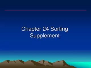
7 4 9 6 2 2 4 6 7 9 4 2 2 4 7 9 7 9 2 2 9 9 Quick-Sort
Quick-Sort x • Quick-sort is a randomized sorting algorithm based on the divide-and-conquer paradigm: • Divide: pick a random element (called pivot) and partition into • - elements less than • - elements equal • - elements greater than • Recur: sort and • Conquer: join , , and x L G E x
Partition • We partition an input sequence as follows: • We remove, in turn, each element from and • We insert into , , or , depending on the result of the comparison with the pivot Algorithm Input: Sequence , position of the pivot Output: Subsequences of the elements of less than, equal to, or greater than the pivot, respectively • while • if • else if • else // • return
Quick-Sort Tree • An execution of quick-sort is depicted by a binary tree • Each node represents a recursive call of quick-sort and stores • Unsorted sequence before the execution and its pivot • Sorted sequence at the end of the execution • The root is the initial call • The leaves are calls on subsequences of size 0 or 1 7 4 9 6 2 2 4 6 7 9 4 2 2 4 7 9 7 9 2 2 9 9
Execution Example • Pivot selection 7 2 9 4 3 7 6 1 1 2 3 4 6 7 7 9 2 4 3 1 1 2 3 4 7 9 77 7 9 4 33 4 9 9 1 1 4 4
Execution Example • Partition, recursive call, pivot selection 7 2 9 4 3 7 6 1 1 2 3 4 6 7 7 9 2 4 3 1 1 2 3 4 7 9 77 7 9 4 33 4 9 9 1 1 4 4
Execution Example • Partition, recursive call, base case 7 2 9 4 3 7 6 1 1 2 3 4 6 7 7 9 2 4 3 1 1 2 3 4 7 9 77 7 9 4 33 4 9 9 1 1 4 4
Execution Example • Recursive call, …, base case, join 7 2 9 4 3 7 6 1 1 2 3 4 6 7 7 9 2 4 3 1 1 2 3 4 7 9 77 7 9 4 33 4 9 9 1 1 4 4
Execution Example • Recursive call, pivot selection 7 2 9 4 3 7 6 1 1 2 3 4 6 7 7 9 2 4 3 1 1 2 3 4 7 9 77 7 9 4 33 4 9 9 1 1 4 4
Execution Example • Partition, …, recursive call, base case 7 2 9 4 3 7 6 1 1 2 3 4 6 7 7 9 2 4 3 1 1 2 3 4 7 9 77 7 9 4 33 4 9 9 1 1 4 4
Execution Example • Join, join 7 2 9 4 3 7 6 1 1 2 3 4 6 7 7 9 2 4 3 1 1 2 3 4 7 9 77 7 9 4 33 4 9 9 1 1 4 4
In-Place Quick-Sort • Quick-sort can be implemented to run in-place • In the partition step, we use replace operations to rearrange the elements of the input sequence such that • the elements less than the pivot have indices less than • the elements equal to the pivot have indices between and • the elements greater than the pivot have indices greater than • The recursive calls consider • elements with indices less than • elements with indices greater than Algorithm Input: Array , indices Output: Array with the elements between and sorted • if • return • //random integer between and • return
In-Place Partitioning • Perform the partition using two indices to split into and (a similar method can split into and ). • Repeat until and cross: • Scan to the right until finding an element . • Scan to the left until finding an element . • Swap elements at indices and j k 3 2 5 1 0 7 3 5 9 2 7 9 8 9 7 6 9 (pivot = 6) 3 2 5 1 0 7 3 5 9 2 7 9 8 9 7 6 9
Analysis of Quick Sort using Recurrence Relations • Assumption: random pivot expected to give equal sized sub-lists • The running time of Quick Sort can be expressed as: • - time to run on input of size Algorithm Input: Sequence , indices Output: Sequence with the elements between and sorted • if • return • //random integer between and • return
Analysis of Partition • Each insertion and removal is at the beginning or at the end of a sequence, and hence takes time • Thus, the partition step of quick-sort takes time Algorithm Input: Sequence , position of the pivot Output: Subsequences of the elements of less than, equal to, or greater than the pivot, respectively • while • if • else if • else // • return
So, the expected complexity of Quick Sort • Assumption: random pivot expected to give equal sized sub-lists • The running time of Quick Sort can be expressed as: Algorithm Input: Sequence , indices Output: Sequence with the elements between and sorted • if • return • //random integer between and • return
Worst-case Running Time • The worst case for quick-sort occurs when the pivot is the unique minimum or maximum element • One of and has size and the other has size • The running time is proportional to: • Alternatively, using recurrence equations: …
1 2 3 4 5 6 7 8 9 10 11 12 13 14 15 16 Expected Running Timeremoving equal split assumption • Consider a recursive call of quick-sort on a sequence of size • Good call: the sizes of and are each less than • Bad call: one of and has size greater than • A call is good with probability 1/2 • 1/2 of the possible pivots cause good calls: 7 2 9 4 3 7 6 1 9 7 2 9 4 3 7 6 1 1 7 2 9 4 3 7 6 2 4 3 1 7 9 7 6 Bad call Good call Bad pivots Bad pivots Good pivots
Expected Running Time • Probabilistic Fact: The expected number of coin tosses required in order to get heads is (e.g., it is expected to take 2 tosses to get heads) • For a node of depth , we expect • ancestors are good calls • The size of the input sequence for the current call is at most • Therefore, we have • For a node of depth , the expected input size is one • The expected height of the quick-sort tree is • The amount or work done at the nodes of the same depth is • Thus, the expected running time of quick-sort is
Comparison-Based Sorting • Many sorting algorithms are comparison based. • They sort by making comparisons between pairs of objects • Examples: bubble-sort, selection-sort, insertion-sort, heap-sort, merge-sort, quick-sort, ... • Let us therefore derive a lower bound on the running time of any algorithm that uses comparisons to sort elements, . Is ? no yes
Counting Comparisons • Let us just count comparisons then. • Each possible run of the algorithm corresponds to a root-to-leaf path in a decision tree
Decision Tree Height • The height of the decision tree is a lower bound on the running time • Every input permutation must lead to a separate leaf output • If not, some input …4…5… would have same output ordering as …5…4…, which would be wrong • Since there are leaves, the height is at least
The Lower Bound • Any comparison-based sorting algorithm takes at least time • That is, any comparison-based sorting algorithm must run in )time.
Bucket-Sort and Radix-Sort 1, c 3, a 3, b 7, d 7, g 7, e 0 1 2 3 4 5 6 7 8 9 Can we sort in linear time? B