Download
1 / 48
480 likes | 589 Views
The informatics of SNPs and haplotypes. CGDN Bioinformatics Workshop June 25, 2007. Gabor T. Marth. Department of Biology, Boston College marth@bc.edu. cause inherited diseases. allow tracking ancestral human history. Why do we care about variations?. underlie phenotypic differences.

E N D
The informatics of SNPs and haplotypes CGDN Bioinformatics Workshop June 25, 2007 Gabor T. Marth Department of Biology, Boston College marth@bc.edu
cause inherited diseases allow tracking ancestral human history Why do we care about variations? underlie phenotypic differences
look at multiple sequences from the same genome region • use base quality values to decide if mismatches are true polymorphisms or sequencing errors How do we find sequence variations?
Sequence clustering Cluster refinement Multiple alignment SNP detection Steps of SNP discovery
Two innovative ideas: 1. Utilize the genome reference sequence as a template to organize other sequence fragments from arbitrary sources 2. Use sequence quality information (base quality values) to distinguish true mismatches from sequencing errors sequencing error true polymorphism Computational SNP mining – PolyBayes
SNP mining steps – PolyBayes sequence clustering simplifies to database search with genome reference multiple alignment by anchoring fragments to genome reference paralog filtering by counting mismatches weighed by quality values SNP detection by differentiating true polymorphism from sequencing error using quality values
1. Fragment recruitment (database search) 2. Anchored alignment 3. Paralog identification 4. SNP detection SNP discovery with PolyBayes genome reference sequence
Polymorphism discovery SW Marth et al. Nature Genetics 1999
Genotyping by sequence • SNP discovery usually deals with single-stranded (clonal) sequences • It is often necessary to determine the allele state of individuals at known polymorphic locations • Genotyping usually involves double-stranded DNA the possibility of heterozygosity exists • there is no unique underlying nucleotide, no meaningful base quality value, hence statistical methods of SNP discovery do not apply
Homozygous C HeterozygousC/T HomozygousT Het detection = Diploid base calling Automated detection of heterozygous positions in diploid individual samples
genome reference EST WGS BAC ~ 8 million Sachidanandam et al. Nature 2001 Large SNP mining projects
Variation structure is heterogeneous chromosomal averages polymorphism density along chromosomes
What explains nucleotide diversity? G+C nucleotide content CpG di-nucleotide content recombination rate 3’ UTR 5.00 x 10⁻⁴ 5’ UTR 4.95 x 10⁻⁴ Exon, overall 4.20 x 10⁻⁴ Exon, coding 3.77 x 10⁻⁴ synonymous 366 / 653 non-synonymous 287 / 653 functional constraints Variance is so high that these quantities are poor predictors of nucleotide diversity in local regions hence random processes are likely to govern the basic shape of the genome variation landscape (random) genetic drift
TAACAAT • mutations are propagated down through generations MRCA TAAAAAT TAAAAAT TAACAAT TAAAAAT TAAAAAT TAACAAT TAACAAT TAACAAT • and determine present-day variation patterns Where do variations come from? • sequence variations are the result of mutation events TAAAAAT
3’ UTR 5.00 x 10⁻⁴ 5’ UTR 4.95 x 10⁻⁴ Exon, overall 4.20 x 10⁻⁴ Exon, coding 3.77 x 10⁻⁴ synonymous 366 / 653 non-synonymous 287 / 653 functional constraints • the genome shows signals of selection but on the genome scale, neutral effects dominate Neutrality vs. selection • selective mutations influence the genealogy itself; in the case of neutral mutations the processes of mutation and genealogy are decoupled
MRCA MRCA accgctatgtaga accgttatgtaga accgctatataga actgttatgtaga SNP density • there is evidence for regional differences in observed mutation rates in the genome CpG content Mutation rate • higher mutation rate (µ) gives rise to more SNPS
large (effective) population size N Long-term demography small (effective) population size N • different world populations have varying long-term effective population sizes (e.g. African N is larger than European)
unique unique Population subdivision shared • geographically subdivided populations will have differences between their respective variation structures
accgttatgtaga acggttatgtaga accgttatgtaga acggttatgtaga accgttatgtaga acggttatgtaga Recombination accgttatgtaga accgttatgtaga acggttatgtaga acggttatgtaga
acggttatgtaga acggttatgtaga acggttatgtaga accgttatgtaga acggttatgtaga acggttatgtaga accgttatgtaga acggttatgtaga acggttatgtaga accgttatgtaga Recombination accgttatgtaga accgttatgtaga acggttatgtaga • recombination has a crucial effect on the association between different alleles
Modeling genetic drift: Genealogy randomly mating population, genealogy evolves in a non-deterministic fashion present generation
Modeling genetic drift: Mutation mutation randomly “drift”: die out, go to higher frequency or get fixed
Modulators: Natural selection negative (purifying) selection positive selection the genealogy is no longer independent of (and hence cannot be decoupled from) the mutation process
Modeling ancestral processes “forward simulations” the “Coalescent” process By focusing on a small sample, complexity of the relevant part of the ancestral process is greatly reduced. There are, however, limitations.
Models of demographic history bottleneck stationary collapse expansion past history present MD (simulation) AFS (direct form)
2. allele frequency spectrum (AFS): distribution of SNPs according to allele frequency in a set of samples “common” “rare” Data: polymorphism distributions 1. marker density (MD): distribution of number of SNPs in pairs of sequences
computable formulations 1/5 2/5 3/5 Model: processes that generate SNPs simulation procedures
Models of demographic history bottleneck stationary collapse expansion past history present MD (simulation) AFS (direct form)
Data fitting: marker density • best model is a bottleneck shaped population size history N3=11,000 N2=5,000 T2=400 gen. N1=6,000 T1=1,200 gen. present Marth et al. PNAS 2003 • our conclusions from the marker density data are confounded by the unknown ethnicity of the public genome sequence we looked at allele frequency data from ethnically defined samples
model consensus: bottleneck N3=10,000 N2=2,000 T2=400 gen. N1=20,000 T1=3,000 gen. present Data fitting: allele frequency • Data from other populations?
bottleneck modest but uninterrupted expansion Population specific demographic history European data African data Marth et al. Genetics 2004
genealogy + mutations allele structure arbitrary number of additional replicates Model-based prediction computational model encapsulating what we know about the process
contribution of the past to alleles in various frequency classes average age of polymorphism Prediction – allele frequency and age European data African data
Allelic association • allelic association is the non-random assortment between alleles i.e. it measures how well knowledge of the allele state at one site permits prediction at another functional site marker site • significant allelic association between a marker and a functional site permits localization (mapping) even without having the functional site in our collection • by necessity, the strength of allelic association is measured between markers • there are pair-wise and multi-locus measures of association
D=f( ) – f( ) x f( ) Linkage disequilibrium • LD measures the deviation from random assortment of the alleles at a pair of polymorphic sites • other measures of LD are derived from D, by e.g. normalizing according to allele frequencies (r2)
strong association: most chromosomes carry one of a few common haplotypes – reduced haplotype diversity Haplotype diversity • the most useful multi-marker measures of associations are related to haplotype diversity n markers 2n possible haplotypes random assortment of alleles at different sites
Haplotype blocks Daly et al. Nature Genetics 2001 • experimental evidence for reduced haplotype diversity (mainly in European samples)
if the block structure is a general feature of human variation structure, whole-genome association studies will be possible at a reduced genotyping cost • this motivated the HapMap project Gibbs et al. Nature 2003 The promise for medical genetics • within blocks a small number of SNPs are sufficient to distinguish the few common haplotypes significant marker reduction is possible CACTACCGA CACGACTAT TTGGCGTAT
The HapMap initiative • goal: to map out human allele and association structure of at the kilobase scale • deliverables: a set of physical and informational reagents
SNPs: computational candidates where both alleles were seen in multiple chromosomes • genotypes: high-accuracy assays from various platforms; fast public data release HapMap physical reagents • reference samples: 4 world populations, ~100 independent chromosomes from each
A C G C T T C A Informational: haplotypes • the problem: the substrate for genotyping is diploid, genomic DNA; phasing of alleles at multiple loci is in general not possible with certainty • experimental methods of haplotype determination (single-chromosome isolation followed by whole-genome PCR amplification, radiation hybrids, somatic cell hybrids) are expensive and laborious
Maximum likelihood approach: estimate haplotype frequencies that are most likely to produce observed diploid genotypes Excoffier & Slatkin Mol Biol Evol 1995 • Bayesian methods: estimate haplotypes based on the observed diploid genotypes and the a priori expectation of haplotype patterns informed by Population Genetics Stephens et al. AJHG 2001 Haplotype inference • Parsimony approach: minimize the number of different haplotypes that explains all diploid genotypes in the sample Clark Mol Biol Evol 1990
Haplotype inference http://pga.gs.washington.edu/
LD-based multi-marker block definitions requiring strong pair-wise LD between all pairs in block Haplotype annotations – LD based Wall & Pritchard Nature Rev Gen 2003 • Pair-wise LD-plots
Dynamic programming approach Zhang et al. AJHG 2001 1. meet block definition based on common haplotype requirements 2. within each block, determine the number of SNPs that distinguishes common haplotypes (htSNPs) 3 3 3 3. minimize the total number of htSNPs over complete region including all blocks Annotations – haplotype blocks
Haplotype tagging SNPs (htSNPs) Find groups of SNPs such that each possible pair is in strong LD (above threshold). Carlson AJHG 2005