BFS preconditioning for high locality, data parallel BFS algorithm
BFS preconditioning for high locality, data parallel BFS algorithm. N.Vasilache , B. Meister, M. Baskaran , R.Lethin. Problem. Streaming Graph Challenge Characteristics: Large scale Highly dynamic Scale-free Massive parallelism, data movement and synchronization is key

BFS preconditioning for high locality, data parallel BFS algorithm
E N D
Presentation Transcript
BFS preconditioning for high locality, data parallel BFS algorithm N.Vasilache, B. Meister, M. Baskaran, R.Lethin
Problem • Streaming Graph Challenge Characteristics: • Large scale • Highly dynamic • Scale-free • Massive parallelism, data movement and synchronization is key • Completely unpredictable • In this talk, focusing on breadth-first search
Breadth-First Search • Dynamic exploration algorithm: • Computes a single source shortest path • O (V + E) complexity -> important • First graph500 problem • Comes in a variety of base implementation: • sequential list • sequential csr, ompcsr • mpi • MTGL • Best 2010 implementation is IBM’s MPI • We propose a solution to optimize the run of a single BFS (graph500 requirement). Rely on a test run, BFS_0 to precondition placement, locality and parallelism.
High-Level Ideas • Assume the result of a first BFS run is available (BFS_0) • In the form provided by graph500 (list of fathers or -1 if root) • BFS_0 can be viewed as an ordering (a traversal) of connected vertices consistent with an ordering of the edges. • Construct a representation that exploits BFS_0 • Parallel distributed construction • Data parallel programming idioms • Reuse the representation for subsequent BFS runs • Improve parallelism and locality • Must be profitable including the overhead of the representation • Must bring improvement on a single BFS run (graph500 requirement) • Very preliminary work
BFS_0 interesting properties • In BFS_0 order: siblings are contiguous, children are localized (recursively), parent is not too far, potential neighbors not too far • Given a graph and a potential BFS: • Full edges are actually used in BFS, dashed edges are potential edges, red dashed edges are illegal edges
BFS_0 interesting properties (continued) • Additional “structural information” on the graph carried by BFS_0 • Potential neighbors of “f” are in the grey region • Distance between “f” and “d” is 1 or 2 at most • Clear separation of potential vertices in 3 classes depending on the depth in BFS_0 relative to the depth of “f”
Sketch of proposed algorithm • We want to reuse as much information from BFS_0 as possible • Given 1 visited node “N”, 3 classes are really data independent regions (-1 depth, same depth, +1 depth) • Additionally, we distinguish Children of N from other Nephew nodes
Sketch of proposed algorithm • We give highest importance to NChildren relation: • position of first child > position of any node in {PlusOne – Children} simple criterion for parallel processing • Children are contiguous, Nephews are not • visiting Children in the BFS_0 order must be stable under recursion • suppose I want a shortest path from i to g: • ibg is impossible • idg is ok but lacks structure • ifg is much better (recursively contiguous and data parallel) • Children are important, we hope there many
Sketch of proposed algorithm • “Discover-and-Merge-and-Mark” algorithm • Given a single starting node we can explore 4 regions in parallel (C,P,S,M) • Order of commit is M,S,P,C • for a node at distance 2 from N and at same depth as N in BFS_0, a transition MC must be favored over a transition SS • This order guarantees recursive consistency of children relation • In general, nodes should be marked in the BFS_0 order • Order of commit is relevant for nodes discovered at the same distance and same depth in BFS_0 wrt the starting node • 3 parameters to order traversal: distance, depth, list of transitions lattice of transitions and synchronizations
Lattice of Transitions D=0 Start Node D=1 d=-1 d=0 d=1 D=2 d=-2 d=-1 d=0 d=1 d=2 D=3 d=-3 d=-2 d=-1 d=0 d=1 d=2 d=3 • Let height the height of BFS_0, the maximal distance is 2*height • Maximal depth difference is [-height, height] (can be refined) • Arrows represent producer/consumer dependences: • 2-D and uniform dependences pipelined parallelism (for free !) • Transitions and edge direction are related: • Bottom-Left edge is an M transition ([D,d] [D+1, d-1]) • Vertical edge is an S transition ([D,d] [D+1, d]) • Bottom-Right edge is a (C | P) transition ([D,d] [D+1, d+1])
Available Parallelism D=0 Start Node D=1 d=-1 d=0 d=1 D=2 d=-2 d=-1 d=0 d=1 d=2 D=3 d=-3 d=-2 d=-1 d=0 d=1 d=2 d=3 • Little less constrained than real pipelined parallelism • Some tasks have only 1 or 2 predecessors, relaxed ordering • CPSM transitions allow inter-region parallelism and gives a third dimension of parallelism/synchronizations: • Unable to exploit it yet (need dynamic dependences otherwise too many empty tasks are created)
Overhead Representation From BFS_0 • Graph500 output: • bfs_0_list (for each vertex his father) • xadj (list of edges in compact array) • xoff (for each node, offset of first and last edge in xadj) • Overhead representation we propose: • bfs_order (for each vertex id, the order it was discovered) slight extension of original seq-csr • bfs_0_list (for each position in BFS_0, get the vertex id) sort (used for finalization, maybe not needed) • bfs_0_list_of_positions (for each vertex id, get the list of positions) • num_children(tmp, doall), ordered_num_children(tmp, doall), pps_num_children(PPS, implemented sequentially), pps_depths (PPS) • xoff + xadjwrt BFS_0 (doall + PPS), categorized in v2 (doall) • Takes as much as 1 sequential run at the moment
Implementation • CnC and C++ implementation: • Pointers to helper data structures • All discovered nodes are copied using data collections • CnC task granularity is a pair (D,d): • Generate exactly height * (2*height + 1) / 2 tasks • Synchronization is easy to write: • Each tasks gets input from its predecessors at (D-1, d-1) and/or (D-1,d) and/or (D-1,d+1) • Each tasks puts data at (D,d) • Within a CnC task: • Get input from (D-1, d-1), discover/mark C transition, discover/mark P transition. Get input from (D-1, d), discover/mark S transition. Get input from (D-1, d+1), discover/mark M transition.
Implementation (continued) • Within a CnC task, everything is sequentialized: • Ability to spawn asynchronous tasks would be useful • Very coarse-grained parallelism (1 task is 4 regions, each region may touch many elements in parallel) • 2 implementations: • “intvec” uses the list of edges in the original graph • “intvec.cat” categorizes the edges by region for faster region traversal • A lot of untunedoverhead • Slowdown … but still valuable information
Statistical Analysis • Biggest example I ran ("size 22" in graph500 terminology): • Scale free graph, 4M vertices and 88M edges • The height of the BFS tree is only 7 small world property • The total number of CnCtasks created is only 14*7 / 2 = 49 • Of these 49 tasks, only a fraction actually perform work, maybe 10 • The work performed is extremely unbalanced: • one task can discover up to 1M new nodes • others discover only 1. • ~70% of discovery and marks happen by visiting C transitions • children are all contiguous in BFS_0 which gives great locality • children have good synchronization properties: they can all be processed in parallel • Need to spawn subtasks
Another Implementation • There is literally almost no parallelism exploited, but a lot is available • Spawn async tasks • Reduce+prefixto deal efficiently with large C regions • Tried another implementation: • CnC task is now (D, d, last_transition) • For each (D,d), fan-out 4 “discover” tasks CP // S // M • For each (D,d), reduce 1 “merge-and-mark” task dependent on these 4 tasks • Additionally, each discover task can be broken down into a static number of pieces to try and process in parallel • VERY crude way of representing async and prefix-reduction • Huge overhead (between 2 and 4x over the previous CnC version)
Future Work Examine overhead (memory leaks, spurious copies, inefficient hashing, too many tasks created, no dependence specified etc) Hierarchical parallelism Distributed implementation Complement with DFS preconditioning (all recursive children become contiguous)