
Excitation Response Spectrum Analysis Using Femap and Nastran
E N D
Presentation Transcript
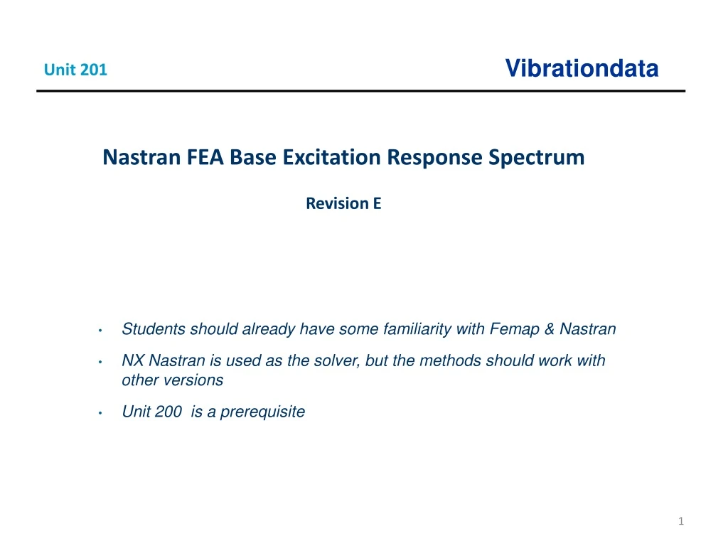
Unit 201 Nastran FEA Base Excitation Response Spectrum Revision E Students should already have some familiarity with Femap & Nastran NX Nastran is used as the solver, but the methods should work with other versions Unit 200 is a prerequisite
Introduction • Shock and vibration analysis can be performed either in the frequency or time domain • Continue with plate from Unit 200 • Aluminum, 12 x 12 x 0.25 inch • Translation constrained at corner nodes • Mount plate to heavy seismic mass via rigid links • Use response spectrum analysis • SRS is “shock response spectrum” • Compare results with modal transient analysis from Unit 200 • The following software steps must be followed carefully, otherwise errors will result Rigid links
Procedure, part I • Femap, NX Nastran and the Vibrationdata Matlab GUI package are all used in this analysis • The GUI package can be downloaded from: https://vibrationdata.wordpress.com/ • The mode shapes are shown on the next several slides for review
Femap: Mode Shape 1 • The fundamental mode at 117.6 Hz has 93.3% of the total modal mass in the T3 axis • The acceleration response also depends on higher modes
Femap: Mode Shape 6 • The sixth mode at 723 Hz has 3.6% of the total modal mass in the T3 axis • This mode has the highest contribution to the T3 peak acceleration response at the center node to the input shock • This partly is because there is more input energy at this frequency than at the fundamental frequency and also this mode has the highest eigenvector response at the center node
Femap: Mode Shape 12 • The twelfth mode at 1502 Hz has 1.6% of the total modal mass in the T3 axis
Femap: Mode Shape 19 • The 19th mode at 2266 Hz has only 0.3% of the total modal mass in the T3 axis • But it still makes a significant contribution to the acceleration response
Matlab: Node 1201 Parameters for T3 • The Participation Factors & Eigenvectors are shown as absolute values • The Eigenvectors are mass-normalized • Modes 1, 6, 12 & 19 account for 98.9% of the total mass
Procedure, part II • Response spectrum analysis is actually an extension of normal modes analysis • ABSSUM – absolute sum method • SRSS – square-root-of-the-sum-of-the-squares • NRL – Naval Research Laboratory method • The SRSS method is probably the best choice for response spectrum analysis because the modal oscillators tend to reach their respective peaks at different times according to frequency • The lower natural frequency oscillators take longer to peak
ABSSUM Method • Conservative assumption that all modal peaks occur simultaneously Pick D values directly off of Relative Displacement SRS curve where is the mass-normalized eigenvector coefficient for coordinate i and mode j These equations are valid for both relative displacement and absolute acceleration.
SRSS Method Pick D values directly off of Relative Displacement SRS curve These equations are valid for both relative displacement and absolute acceleration.
Femap: Constraints • The response spectrum setup has some similarities and differences relative to modal transient • Delete all constraints, functions, and output sets from previous model • Delete the base mass and rigid links if present • Delete all unused nodes • Resume as follows: • Create constraint set call seismic & edit corner node constraints so that only TX & TY are fixed
Femap: Added Points and Nodes Node 2402 Node 2403 • Copy center point twice at -3 inch increments in the Z-axis • Place nodes on added points
Femap: Mass • Calculate FEA model mass • Select all elements • Result is 0.00913968 lbf sec^2/in • Or 1.6 kg • Copy total mass using Ctrl-C
Femap: Seismic Mass • Define Seismic Mass property • Mass value is model mass x 1e+06 • Enter the following number in the mass box 0.00913968*1e+06 • The edit box is too small to show complete number
Femap: Seismic Mass Placement Node 2403, Seismic Mass
Femap: Rigid Link no. 1, TZ only • Four corner nodes are dependent Node 2402, Independent
Femap: Rigid Link no. 2, TZ only Node 2402, Dependent Node 2403, Independent
Femap: Add Constraints to Current Constraint Set All DOF fixed except TZ
Femap: Add Constraint to Kinematic Set Constrain TZ • The seismic mass is constrained in TZ which is the response spectrum base drive axis
Femap: Define Damping Function • Q=10 is the same as 5% Critical Damping
Shock Response Spectrum Q=10 • Good practice to extrapolate specification down to 10 Hz if it begins at 100 Hz • Because model may have modes below 100 Hz • Aerospace SRS specifications are typically log-log format • So good practice to perform log-log interpolation as shown in following slides • Go to Matlab Workspace and type: • >> spec=[10 10; 2000 2000; 10000 2000]
Matlab: Export Data >> spec=[10 10; 2000 2000; 10000 2000] • Multiply by 386 to convert G to in/sec^2 • Save as: srs_Q10.bdf or whatever
Femap: View Response Spectrum Function • Change title from TABLED2 to SRS_Q10
Femap: Define Response Function vs. Critical Damping • For simplicity, the model damping and SRS specification are both Q=10 or 0.05 fraction critical • Function 7 is the SRS specification • Specifications for other damping values could also be entered as functions and referenced in this table, as needed for interpolation if the model has other damping values • Multiple SRS specifications is covered in Unit 202
Femap: Define Normal Modes Analysis Parameters • Solve for 20 modes
Femap: SRS Cross-Reference Function This is the function that relates the SRS specifications to their respective damping cases “Square root of the sum of the squares” The responses from modes with closely-spaced frequencies will be lumped together
Femap: Define Boundary Conditions Main Constraint function Base input constraint, TZ for this example
Femap: Define Outputs • Quick and easy to output results at all nodes & elements for response spectrum analysis • Only subset of nodes & elements was output for modal transient analysis due to file size and processing time considerations Get output f06 file
Femap: Export Nastran Analysis File • Export analysis file • Run in Nastran
Matlab: Response Spectrum Acceleration Results • Center node 1201 has T3 peak acceleration = 475.9 G from response spectrum analysis • Modal transient result from Unit 200 was 461 G for this node
Matlab: Response Spectrum Acceleration Results (cont) Node 49 Node 1201 • Center node 1201 had T3 peak acceleration = 475.9 G • Edge node 49 had highest T3 peak acceleration = 612.5 G • By symmetry, three other edge nodes should have this same acceleration • But node 1201 had highest displacement and velocity responses
Matlab: Response Spectrum Results Maximum accelerations: node value T1: 2376 0.000 G T2: 931 0.000 G T3: 49 612.541 G R1: 1 116739.700 rad/sec^2 R2: 1 116739.700 rad/sec^2 R3: 1 0.000 rad/sec^2 Maximum Displacements: node value T1: 2376 0.00000 in T2: 931 0.00000 in T3: 1201 0.10746 in R1: 1 0.02054 rad/sec R2: 1 0.02054 rad/sec R3: 1 0.00000 rad/sec Maximum Quad4 Stress: element value NORMAL-X : 1105 6047.053 psi NORMAL-Y : 24 6047.053 psi SHEAR-XY : 50 4798.865 psi MAJOR PRNCPL: 24 6047.816 psi MINOR PRNCPL: 1128 4997.801 psi VON MISES : 50 8400.833 psi Maximum velocities: node value T1: 2376 0.000 in/sec T2: 931 0.000 in/sec T3: 1201 83.665 in/sec R1: 1 20.246 rad/sec R2: 1 20.246 rad/sec R3: 1 0.000 rad/sec
Acceleration Response Check for Node 1201 T3 • Center node 1201 had T3 peak acceleration = 475.9 G from the FEA • The FEA value passes the modal combination check
Vibrationdata SRS Modal Combination >> spec=[10 10; 2000 2000; 10000 2000]
Vibrationdata SRS Modal Combination Results SRS Q=10 fn(Hz) Accel(G) 10.0 10.0 2000.0 2000.0 10000.0 2000.0 fnQ=10 (Hz) SRS(G) 117.6 117.6 723.6 723.6 1502 1502 2266 2000 fn Part Eigen SRS Modal Response (Hz) Factor vector Accel(G) Accel(G) 117.6 0.0923 13.98 117.6 151.7 723.6 0.0182 -22.28 723.6 293.4 1502 0.0123 2.499 1502 46.17 2266 0.0053 32.2 2000 341.3 ABSSUM= 832.7 G SRSS= 477.2 G
Acceleration Response Check for Node 49 T3 • Edge node 49 had T3 peak acceleration = 612.5 G from the FEA • The FEA value passes the modal combination check
Femap: T3 Acceleration Contour Plot, unit = in/sec^2 • Import the f06 file into Femap and then View > Select