Download
1 / 35
350 likes | 373 Views
Explore parallel techniques such as partitioning, pipelining, synchronous, and asynchronous computations to achieve load balancing. Discover practical applications like low-level image processing and Mandelbrot set calculations. Parallelize Mandelbrot set computation with static task assignment for improved efficiency. Dive into examples of parallelizing image operations and understand the benefits of divide-and-conquer approaches in cluster computing.

E N D
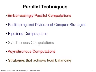
Parallel Techniques • Embarrassingly Parallel Computations • Partitioning and Divide-and-Conquer Strategies • Pipelined Computations • Synchronous Computations • Asynchronous Computations • Strategies that achieve load balancing 3.1 Cluster Computing, UNC-Charlotte, B. Wilkinson, 2007.
Embarrassingly Parallel Computations A computation that can obviously be divided into a number of completely independent parts, each of which can be executed by a separate process(or). No communication or very little communication between processes Each process can do its tasks without any interaction with other processes 3.3
Practical embarrassingly parallel computation with static process creation and master-slave approach 3.4
Embarrassingly Parallel Computation Examples • Low level image processing • Mandelbrot set • Monte Carlo Calculations 3.6
Low level image processing Many low level image processing operations only involve local data with very limited if any communication between areas of interest. 3.7
Image coordinate system Origin (0,0) x . (x, y) y 3.9
Some geometrical operations Shifting Object shifted by Dx in x-dimension and Dy in y-dimension: x¢ = x + Dx y¢ = y + Dy where x and y are original coordinates and x¢ and y¢ are the new coordinates. x y Dx Dy 3.8
Some geometrical operations Scaling Object scaled by factor Sxin x-direction and Syin y-direction: x¢ = xSx y¢ = ySy x y 3.8
Rotation Object rotated through an angle q about the origin of the coordinate system: x¢ = x cosq + y sinq y¢ = -x sinq + y cosq x y 3.8
Parallelizing Image Operations Partitioning into regions for individual processes Example Square region for each process (can also use strips) 3.9
Mandelbrot Set Set of points in a complex plane that are quasi-stable (will increase and decrease, but not exceed some limit) when computed by iterating the function: where zk +1 is the (k + 1)th iteration of complex number: z = a + bi and c is a complex number giving position of point in the complex plane. The initial value for z is zero. 3.10
Mandelbrot Set continued • Iterations continued until magnitude of z is: • Greater than 2 • or • Number of iterations reaches arbitrary limit. • Magnitude of z is the length of the vector given by: 3.10
Sequential routine computing value of one point returning number of iterations structure complex { float real; float imag; }; int cal_pixel(complex c) { int count, max; complex z; float temp, lengthsq; max = 256; z.real = 0; z.imag = 0; count = 0; /* number of iterations */ do { temp = z.real * z.real - z.imag * z.imag + c.real; z.imag = 2 * z.real * z.imag + c.imag; z.real = temp; lengthsq = z.real * z.real + z.imag * z.imag; count++; } while ((lengthsq < 4.0) && (count < max)); return count; } 3.11
Mandelbrot Set The display height is disp_height, the display width is disp_width, and the point in the display area is (x, y). If this window is to display the complex plane within minimum values of (real_min, imag_min) and maximum values of (real_max, imag_max), each (x,y) needs to be scaled by the factors. scale_real = (real_max – real_min) /disp_width; scale_imag = (imag_max – imag_min) / disp_height; for(x = 0; x < disp_width; x++) for (y = 0; y < disp_height; y++) { c.real = real_min + ((float) x * scale_real); c.imag = imag_min + ((float) y * scale_imag); color = cal_pixel(c); display(x, y, color); }
Mandelbrot set http://www.cs.siu.edu/~mengxia/Courses%20PPT/520/mandelbrot.c cc -I/usr/X11R6/include –o mandelbrot mandelbrot.c -L/usr/X11R6/lib64 -lX11 -lm 3.12
Parallelizing Mandelbrot Set Computation Static Task Assignment Simply divide the region in to fixed number of parts, each computed by a separate processor. Each processor needs to execute the procedure, cal_pixel(), after being given the coordinates of the pixels to compute. Suppose the display area is 480x640 and we were to compute 60 rows in a process, a grouping of 60x640 pixels and 8 processors in our Athena cluster. Not very successful because different regions require different numbers of iterations and time. 3.13
Parallel pseudocode Master for (i = 0; row= 0; i< 8; i++, row=row+60) /*for each process*/ send(&row, pi); /*send row number*/ for (i = 0; i< (480*640); i++) { /*from processes, any order */ recv(&c, &color, PANY); display(c, color); } Slave ( process i) recv(&row, Pmaster); /*receive row no. */ for (x=0; x<disp_width; x++) /*screen coordinates x and y*/ for ( y=row; y<(row+60); y++) { c.real = real_min + ((float) x * scale_real); c.imag = imag_min + ((float) y * scale_imag); color = cal_pixel(c); send(&c, &color, Pmaster); /*send coords, color to master*/ }
Analysis • Serial time: ts <= max_iter x n //for n pixels • tcomm1 = (p-1)(tstartup + tdata) // for the first row number • tcomp <= max_iter x n / (p-1) //divide the image into groups of n/(p-1) pixels, each requires at most max_iter steps • tcomm2 = n (tstartup + 3 x tdata) // each pixel has three integers, two for coordinates and one for color • Speedup factor approaches p if max_iter is large.
Dynamic Task Assignment Have processor request regions after computing previous regions 3.14
Each slave is first given one row to compute and, from then on, gets another row when it returns a result, until there are no more rows to compute. • The master sends a terminator message when all the rows have been taken. To differentiate between different messages, tags are used with the message data_tag for rows being sent to the slaves, terminator_tag for the terminator message, and result_tag for the computed results from the slaves.
Master count = 0; /*counter for termination*/ row = 0; /*row being sent*/ For (k=0; k< num_proc; k++) { send ( &row, Pk, data_tag); /*send initial row to process*/ count++; /*count rows sent*/ row++; /*next row*/ } do { recv (&slave, &r, color, PANY, result_tag); count --; /*reduce count as rows received*/ if ( row < dis_height) { send (&row, Pslave, data_tag); /*send next row*/ row++; /*next row*/ count++; } else send (&row, Pslave, terminator_tag); /*terminate*/ display( r, color); /*display row*/ } while (count > 0);
Slave recv( y, Pmaster, ANYTAG, source_tag); /*receive 1st row to compute*/ While (source_tag == data_tag) { c.img = imag.min + ((float) y * scale_imag); for ( x= 0; x< disp_width, x++) { /*compute row colors*/ c.real = real_min ++ ((float) x*scale_real; color [x] = cal_pixel(c); } send (&y, color, Pmaster, result_tag); recv(&y, Pmaster, source_tag); };
Monte Carlo Methods Another embarrassingly parallel computation. Monte Carlo methods use of random selections. 3.15
Circle formed within a 2 x 2 square. Ratio of area of circle to square given by: Points within square chosen randomly. Score kept of how many points happen to lie within circle. Fraction of points within circle will be , given sufficient number of randomly selected samples. 3.16
PI Calculation • The value of PI can be calculated in a number of ways. Consider the following method of approximating PI • Inscribe a circle in a square • Randomly generate points in the square • Determine the number of points in the square that are also in the circle • Let r be the number of points in the circle divided by the number of points in the square • Note that the more points generated, the better the approximation • Serial pseudo code for this procedure: npoints = 10000 circle_count = 0 • do j = 1,npoints • generate 2 random numbers between 0 and 1 xcoordinate = random1 ; ycoordinate = random2 • if (xcoordinate, ycoordinate) inside circle then circle_count = circle_count + 1 • end do • PI = 4.0*circle_count/npoints • Note that most of the time in running this program would be spent executing the loop
Parallel strategy:. For the task of approximating PI: Each task executes its portion of the loop a number of times. • Each task can do its work without requiring any information from the other tasks (there are no data dependencies). • Uses the SPMD model. One task acts as master and collects the results. • Pseudo code solution: • npoints = 10000; circle_count = 0; p = number of tasks; num = npoints/p • find out if I am MASTER or WORKER • do j = 1 to num • generate 2 random numbers between 0 and 1 • xcoordinate = random1; ycoordinate = random2; • if (xcoordinate, ycoordinate) inside circle • then circle_count = circle_count + 1; • end do • if I am MASTER receive from WORKERS their circle_counts compute PI (use MASTER and WORKER calculations) • else if I am WORKER send to MASTER circle_count • endif
Computing an Integral One quadrant can be described by integral Random pairs of numbers, (xr,yr) generated, each between 0 and 1. 3.18
Alternative (better) Method Use random values of x to compute f(x) and sum values of f(x): where xrare randomly generated values of x between x1 and x2. Monte Carlo method very useful if the function cannot be integrated numerically (maybe having a large number of variables) 3.19
Example Computing the integral Sequential Code sum = 0; for (i = 0; i < N; i++) { /* N random samples */ xr = rand_v(x1, x2); /* generate next random value */ sum = sum + xr * xr - 3 * xr; /* compute f(xr) */ } area = (sum / N) * (x2 - x1); Routine randv(x1, x2) returns a pseudorandom number between x1 and x2. 3.20
For parallelizing Monte Carlo code, must address best way to generate random numbers in parallel . Each computation uses a different random number and there is no correlation between the numbers. 3.21
Pseudorandom-number generator • For successful Monte Carlo simulations, the random numbers must be independent of each other. The most popular way of creating a pseudorandom-number sequence is by evaluation x(i+1) from a carefully chosen function of xi. The key is to find a function that will create a large sequence with the correct statistical properties. The linear congruential generator function is of the form: • X(i+1)= (a*xi+c) mod m where a, c and m are constants. Many choices of the constants, a “good” generator is with a=16807, m=2^31 -1 ( a prime number), and c = 0. A repeating sequence of 2^31 -2 different numbers. But it is slow. Numbers are repeatable and deterministic. Being repeatable is god for experiment testing.
Pseudorandom-number generator • Approaches: • Rely on a centralized linear congruential pseudorandom-number generator to send out numbers to slave processes when they request number. Slow and Bottle neck in master node. • Alternatively, each slave can use a separate generator with different formula. If same formula, correlation might occur. Problems: • Even if a random-number generator appears to create a series of random numbers from statistical tests, we cannot assume that different sub-sequence or sampling of numbers from the sequences are not correlated. Generator repeat their sequences at some point.
Pseudorandom-number Generator • A solid parallel versions of pseudorandom-number generator called SPRNG (scalable Pseudorandom Number generator ) is a library specifically for parallel Monte Carlo computations and generate random-number streams for parallel processes. • It has several different generators and features to minimize interprocess correlation. Interface for MPI is also provided. Link to SPRNG packages: • http://www.nersc.gov/nusers/resources/software/libs/math/random/www/index.html • Please use SPRNG to run your Monte Carlo method to compute pi as homework.