OPTIONS
350 likes | 511 Views
OPTIONS. 1. THE TWO BASIC OPTIONS - PUT AND CALL A call (put) is the right to buy (sell) an asset. Most other options are just combinations of these. Options are “derivatives” and other derivatives may include options

OPTIONS
E N D
Presentation Transcript
OPTIONS • 1. THE TWO BASIC OPTIONS - PUT AND CALL • A call (put) is the right to buy (sell) an asset. • Most other options are just combinations of these. • Options are “derivatives” and other derivatives may include options • The price of an option is called a “premium” because options are equivalent to insurance and the price of insurance is called a premium. • 2. For most of this lecture we will assume that the option • a. Can only be exercised at maturity (called European). An American option, which is the most common type should behave similarly because, in most cases, American options are not exercised until maturity. They are almost always worth more left unexercised so very few are exercised. If they are never exercised before expiration, there should be no difference in value between an American and European option. • b. Pays no dividends – most options aren’t dividend protected so dividends will affect price.
Lower Bound for the European Call Option Value is also a Lower Bound for the American Call Option Value • Many of the early results in options were derived using arbitrage arguments. We will not cover all of them here but the lower bound is one example. Consider 2 portfolios A and B: A. Purchase a European call for C with exercise price E and (zero coupon, default free) bonds that will have a value of E at the maturity of the option, i.e., purchase E/(1 + r) amount of bonds B. Purchase the stock at P0 at time 0. Price at expiration is P1. PortfolioActionInvestmentValue at Expiration P1 > E P1 E ABuy call C P1 -E 0 Buy bonds E / (1+r) E E TOTALS C + E / (1+r) P1 E BBuy stockP0P1 P1 if P1 > E then both have same value if P1£ E then Portfolio A is more valuable thus the investment in A must exceed the investment in B or else arbitrage is possible, thus: so
CALL OPTION CONTRACT Definition: The right to purchase 100 shares of a security at a specified exercise price (Strike) during a specific period. EXAMPLE: A January 60 call on Microsoft (at 7 1/2) This means the call is good until the third Friday of January and gives the holder the right to purchase the stock from the writer at $60 / share for 100 shares. Cost is $7.50 / share x 100 shares = $750 premium or option contract price.
PUT OPTION CONTRACT Definition: The right to sell 100 shares of a security at a specified exercise price during a specific period. EXAMPLE: A January 60 put on Microsoft (at 14 1/4) This means the put is good until the third Friday of January and gives the holder the right to sell the stock to the writer for $60 / share for 100 shares. Cost $14.25 / share x 100 shares = $1425 premium.
INTRINSIC AND TIME VALUE • AN OPTION'S INTRINSIC VALUE IS ITS VALUE IF IT WERE EXERCISED IMMEDIATELY. • AN OPTION'S TIME VALUE IS ITS COST ABOVE ITS INTRINSIC VALUE. • Microsoft Stock Price = 53 1/4 at the time - October 1987 • QUESTION: Which Microsoft option has greater intrinsic value? - put • QUESTION: Which Microsoft option has greater time value? – call • QUESTION: Which option is a better deal? • Look at Options Quotes: www.bigcharts.com • COMBINED STRATEGIES • straddle - 1 call and 1 put • strip - 1 call, 2 puts • strap - 2 calls, 1 put • money spread • time spread
OPTIONS EXAMPLES Call - option to buy another company or company's line. Call - capital expenditures on R & D and marketing. Give an option to make further investments if promising. Call - buy car at the end of the lease Call - rain check at a grocery store Put - abandonment Put - agreement to buy company but only if loan losses are less than 50 million (WCIS). Put - guarantees - government price supports - consider farmer's incentives Note: The option pricing model can be used to price any asset for which we can obtain the required inputs. Although stock options are more common, many assets can be priced – often called “real” options.
Call - A stock is a call option on the value of the firm if there is debt in the capital structure. The value of the debt is the strike price. Shareholders exercise their option to own the firm if the firm's value exceeds the value of debt, otherwise, they default and give the firm to the debt-holders. This means that many stock options are actually options on options – pricing is more complex than Black-Scholes. Firm value 10mm 3mm Debt value 5mm3mm EQUITY value 5mm 0mm This situation can also be consider from the bondholders perspective which involves a put option. Put – Bondholders have the equivalent of a risk-free bond and a short position in a put on the company that is given to shareholders. If the value of the firm drops below 5mm, then shareholders put the company to the bondholders so that Risk-free Debt value 5mm 5mm Short put value 0mm -2mm DEBT value 5mm 3mm
USE OPTIONS TO CUT UP PRICE DISTRIBUTIONS - NOW CALLED "FINANCIAL ENGINEERING"
BLACK - SCHOLES MODEL CRUCIAL INSIGHT - it is possible to replicate the payoff to an option by some investment strategy involving the underlying asset and lending or borrowing - like the stock of a leveraged company. Therefore, we should be able to derive the value of an option from the asset price and the interest rate. Bullish --> Long position --> buy 100 shares of stock for, say $10,000 or buy Call option on 100 shares for $1000 and receive interest on $9000. Here the option position has an advantage over the stock position of earning interest. Bearish --> Short position --> sell 100 shares short, put up $1000 margin and earn interest on short sale proceeds or buy Put for $1000. Here the short stock position has an advantage over the option position of earning interest.
THERE IS A HEDGE RATIO BETWEEN THE CALL AND STOCK THAT ESSENTIALLY ALLOWS ONE TO EXACTLY REPLICATE AN OPTION For a simplified approach to replication one can use the Binomial Model. 1. Assume that S = Stock price today C = Call option price today r = risk-free rate q = the probability the stock price will increase (1-q)= the probability the stock price will decrease u = the multiplicative increase (u > 1 + r > 1) d = the multiplicative decrease (0 < d < 1 < 1 + r ) Cu = call price if stock price increases Cd = call price if stock decreases Each period the stock can take on only two values; the stock can move up to uS or down to dS. 2. Construct a risk-free hedge portfolio composed of one share of stock and m call options written against the stock. This means the payoffs in the up or down moves will be the same so that uS – mCu = dS – mCd Solve for m, the hedge ratio of calls to be written on stock m = S(u – d)/(Cu - Cd )
3. Because we constructed the portfolio to be risk-free, then (1 + r)(S – mC) = uS – mCu Or 4. Substituting for the hedge ratio m, Or simplify let and So C = [pCu + (1 - p)Cd] / (1 + r)
Compare C = [pCu + (1 - p)Cd] / (1 + r) to C = [πCu + (1 - π)Cd] / (1 + RAR) Here, p is called the hedging probability, also called the risk-neutral probability. The potential option payoffs Cu and Cd are multiplied by the risk neutral probabilities and the sum is discounted at the risk-free rate. Note: the risk-neutral probability for the up (down) move is less (more) than the objective probability, π, that would be used if we discounted the payoffs with a risk-adjusted rate (RAR from a CAPM rate based on option beta) because the value in the numerator must be smaller if we are discounting at the smaller risk-free rate r.
Relation between That is, p is the value q would take if all investors are risk neutral and thus value the stock as follows, (1 + r)S = quS + (1 – q)dS Solving for q gives Now this probability can be used to discount the payoffs for the call option Cu and Cd. 5. Newer techniques for solving for derivatives prices often employ the risk neutral approach. The risk neutral approach takes advantage of the fact that we can value an option in two ways. One is based upon the assumption that a stock will follow some process where its price drifts upward over time at a rate equal to its expected return. The option is then priced off the stock. The problem is that we don’t have good models of expected returns for the stock or the option (APT and CAPM don’t work well). Instead, one can assume that the stock will increase at the risk-free rate and use the risk-neutral probabilities and discount the future option payoffs at the risk-free rate. That is, we use the wrong expected return for the stock (a risk-free return instead of the risky expected return) and the wrong probabilities (risk neutral probabilities) for the option payoffs, but the errors always just offset.
Relation between the risk neutral and true (physical) probabilities Start as before but with a risk averse investor, and the stock return is R = r + e, where e is the excess return. (1 + R)S = quS + (1 – q)dS Or (1 + r + e)S = quS + (1 – q)dS Solving for q gives This shows that the true probability q is larger than the risk neutral probability p. To get a more formal expression for the relation between p and q, recall that the standard deviation of a binomial is σ = [q(1-q)].5(u-d) Also E(R) = qu + (1-q)d – 1 And B = [E(R) - r]/σ Plug these in above and get p = q - B[q(1-q)].5 So again p < q for risk averse investors, and for risk neutral investors B = 0 so p = q.
Note: The exact call option payoffs can be duplicated with a portfolio of [(Cu - Cd)/(u – d)S] (inverse of m) shares of stock and borrowing [(uCd - dCu)/(u – d)(1 + r)] at the risk-free rate. 6. Interesting features of call formula. a. It does not depend on the probability of an upward movement q (or (1-q)), so heterogeneous expectations by investors about q are no problem because the stock price aggregates heterogeneous expectations about q and the option price is simply derived from the stock price. If the probability of an upward move is large, the current stock price will be higher, all else equal. b. Investors risk preferences are irrelevant to call price derivation since, again the stock price reflects it. c. The only security relevant to the option is the underlying stock; the market portfolio or factors are irrelevant. Again, the stock is priced according to these. d. We are able to perfectly hedge the option with the stock because the returns for the two are perfectly correlated. 7. To get the call price for a two period model, just apply the one period model twice to get. C = [p2Cuu + p(1 - p)Cud + p(1 - p)Cdu + (1 - p)2Cdd ] / (1 + r)2 Where Cuu, Cud = Cdu and Cdd are the three possible values for the option after two periods. For more periods, just use binomial expansion.
Example: Suppose that a stock’s price is S=100 and it can increase by 100% or decrease by 50%. If the risk-free rate is 8% and the exercise price for a call is $125, find the price of the call, the hedge ratio, the risk-neutral probabilities and the amount of stock and risk-free borrowing one needs to replicate call the option. m = 100(2 – .5)/(75 - 0) = 2 Here, the option price moves half as much as the stock’s. Therefore, if you own one share of the stock in this example, you can hedge, that is, eliminate your risk, by selling two calls. And 1 – p = .61333 Duplicate call with [(Cu - Cd)/(u – d)S] = (75 – 0)/(2 - .5)100 = .5 shares of stock And borrow [(uCd - dCu)/(u – d)(1 + r)] = (2(0) - .5(.75))/(2 - .5)(1 + .08) = 23.15
1. To see how hedging works, form a hedged portfolio by buying one share and selling 2 options and find its risk-free end-of-period value. Stock goes: DownUp Own the stock 50 200 Sold 2 options 0-150 50 50 Whatever happens, you get 50 so it is risk-free portfolio, i.e., perfectly hedged. Find the present value of the portfolio’s end value by discounting at the risk-free rate. In this case, 50/(1+.08)=46.30. You borrow this amount of money and add (S – 46.30) = (100 – 46.30) = $53.70 of your own money to buy one share. This leveraged position in the stock should give the same return as owning two calls. To see this note that in one year you pay off the loan and you will have 150 [= 200 - 46.30(1+.08)] if stock goes to 200 or 0 [= 50 - 46.30(1+.08)] if the stock goes to 50.
Set the present value of the hedged portfolio equal to its discounted risk-free value and solve for C. • Here, S - 2 C = 100 - 2C = 46.30 => C=26.85. • 2. Another way to see this for the data above is to consider that • the stock payoff in one period is the combination of a risk free 50 dollars (if you own the stock you know you will have at least 50 in one period) plus the risky payoff of 0 or 150 dollars. • You can finance the position by borrowing 50/(1+r) = 50/(1.08) =46.30 at the risk free rate. A bank holding your security would do this because they know the security will be worth at least 50 in one year to cover the loan. • Of course, to buy the stock at 100 you had to put up 100 – 46.30 = 53.70 of your own money. • We have m=2 as before, which means that the value of your stock plus your borrowing portfolio will move twice as much as the call. This means that you can perfectly hedge a call with half of your stock plus borrowing portfolio. • C = (1/m)[S - dS/(1 + r)] = (1/2)[100 – 50/(1.08)] = 26.85
3. The binomial can also be illustrated using state-specific securities. Note that there are only two states, up or down. The payoffs can be used to determine the two state security prices and then the option can be priced by multiplying the state prices times the units of state securities that make up the option. 4. Finally, we could find the risk neutral probabilities first and then apply them to the two possible outcomes and then discount the total at the risk free rate.
GET THE PUT VALUE - PUT/CALL PARITY FORMULA • Put Price = C - S + E/(1 + risk-free rate)t • For this case: • Put = 26.85 - 100 + 125/(1 + .08)1 = 42.6. • This model shows that, to get an option value, ones needs to know the • current stock price • option’s exercise price • risk-free rate • option maturity • stock price volatility.
Proof of Put-Call Parity Consider two Portfolios A and B: A. Purchase the stock for P0, purchase a put for T0 with exercise price E and borrow E/(1 + r) at the risk-free rate r (in one year at maturity you will have to pay back E). B. Purchase the call at C0 also with exercise E and one year maturity. PortfolioActionInvestmentValue at Expiration P1 > E P1 E ABuy Stock P0 P1 P1 Buy Put T0 0 E - P1 Borrow -E/(1 + r) -E -E TOTALS P0 + T0 - E/(1+r) P1 –E 0 BBuy Call C0P1 - E 0 Both A and B have the same payoff whether P1 > E or P1£ E, therefore, arbitrage arguments imply that both must have the same initial investment. That is, , or for maturity t, If we select E = P0 then This shows that, all else equal, calls sell for more than puts. Why?
BLACK-SCHOLES MODEL - A NEARLY EXACT OPTION PRICING MODEL C0 = P0N(d1) - E e-rt N(d2) where Price of Stock = P0 Exercise price = E Risk free rate = r Time until expiration in years = t Normal distribution function = N( ) Exponential function (base of natural log) = e where: where Standard deviation of stocks return = Natural log function = ln Intuitively, the Black Sholes model can be explained as the discounted expected value of the cash flows at expiration of the option. At expiration, assuming P > E, we pay the exercise price E (a cash outflow) and receive the stock with the value P (a cash inflow). Before expiration, we attach probabilities to these events. The N(d) are probabilities.
This is also a statement of an arbitrage relationship (replicating strategy). The first term, P0N(d1) is the cost of the shares in a portfolio that closely tracks the option value and the second term, E e-rt N(d2) is the amount borrowed at the risk-free rate to partly finance the stock purchase. The difference between the two terms is the value of a call option. N(d2) is the probability that the stock will exceed the option’s exercise price at expiration and N(d1) is the present value of the expected stock price at expiration conditional on P > E times the probability that P > E. The N(d) are cumulative probabilities of a normal distribution. These probabilities are sometimes described as “risk-adjusted” probabilities. For each (d), we have the term ln(P0/E) which is the percent by which the stock price exceeds the exercise price (i.e. is in the money). Clearly, if the stock price exceeds the exercise price by a large percentage, the more likely the call option will be valuable (i.e. exercised) at expiration. But note that ln(P0/E) is divided by t so that the probability is adjusted for the stock’s risk and the time to expiration. A call on a risky stock (relatively large ) that is in the money by a given percent has less probability of staying in the money.
Another way to look at N(d1) is as the partial derivative of call price with respect to stock price. C/P0 = N(d1) This is the instantaneous hedge ratio comparable to the inverse of m in the binomial model. This derivative is referred to as the “Delta” for an option. Tests of the Black-Scholes option pricing model are joint tests of the model and market efficiency. Most tests show strong support, with only deep out-of-the-money options showing any pricing bias.
How Model Variables Impact Options Prices • Stock price – Positively related to call price. • Negatively related to put price. • Exercise price – Negatively related to call price. • Positively related to put price. • Return Stand. Deviation – Positively related to call price. • Positively related to put price. • Maturity – Positively related to call price. • Positively related to put price (usually). • Interest rate – Positively related to call price. • Negatively related to put price. • All but the interest rate effects are clear. To explain the effect of interest rate intuitively, consider the following. • From the call option formula, we have the discounted exercise price enter the equation with a negative sign. This reflects the fact that if we exercise we have to make a cash payment of the exercise price. If interest rates increase, the present value of that payment today falls, so that the call price must rise. • From the put-call parity formula, we see the opposite occurs since, for a put, we will be receiving the exercise price in the future in exchange for the stock if we exercise.
TO GET THE VALUE OF THE CALL, C0 • EXAMPLE: ASSUME • Price of Stock P0 = 36 • Exercise price E = 40 • Risk free rate r = .05 • time period 3 mo. t = .25 • Std Dev of stock return s = .50 • Substitute into d1 and d2. • Substitute d1, d2 and other variables in the main equation • C0 = 36N(-.25) - 40e-.05(.25)N(-.50) • Look up in the normal table for d to get N(d). • here N(d1) = N(-.25) = .4013 • and N(d2) = N(-.50) =.3085 • Substitute in the main equation
USE PUT CALL PARITY FORMULA TO GET PUT PRICE T0 = PUT PRICE To see why this holds, look at the stock price distribution and how the put gives you the left tail of the distribution. Then see that shorting the stock and buying the call leaves you with the same left tail. Or see that payoff at time t=0 is equal on both sides no matter what price is. EXAMPLE - use info above - you need the call price = 2.26 - 36 + 39.5 = 5.76 Put-call parity is acceptable for European puts and usually for American puts of short maturity (< 1 year). However, when the chance of early exercise is relatively large, for example, for long maturity puts, put prices are derived using computerized numerical methods. The main reason is that if the underlying stock price were to fall to very low levels (think internet stocks) then it pays to exercise early. Time becomes a negative there because the most that you can gain by holding is for the stock to fall to zero, but by waiting, the stock still has unlimited upside. It is then best to exercise an American put early.
NET PRESENT VALUE RULE FOR PROJECT ACCEPTANCE MUST BE ADJUSTED IF OPTIONS ARE INVOLVED. There are two types of options to consider for most projects A. The call option to delay a project to the future when the project may have a larger NPV. A project that can be delayed effectively competes with itself in the future. This call option is more valuable when a project can be delayed for a longer time (t), when a project’s (returns) are very risky (s), and when interest rates (r) are high. This could explain why it may be rational to delay a positive NPV project; Managers have often been criticized by governments for not investing in plant and equipment during recessions. Managers are not being indecisive or too risk-averse but simply evaluating projects based upon their option values which may be high during recessions. The basic idea is that if you undertake a project now, you can’t undertake it in the future when it may have a higher NPV. The more likely a project could have a higher NPV in the future, the larger its option’s time value. If the project is accepted, its time value is lost.
Thus, time value must be considered in the project selection criteria. Thus instead of NPVproject > 0 we use NPVproject > time value of the option to delay > 0 Hence we should accept a project only when it has a relatively large NPV. A large NPV in options terms means that the market value or present value of the project’s cash flows greatly exceeds its exercise price (cost of the project). In other words - when its option is sufficiently “in the money” i.e., it has much intrinsic value.
B. When a project’s acceptance allows one to undertake additional projects in the future then we must make another adjustment to the NPV criteria above. NPVproject + Value of option on extended projects > time value of option to delay For example, if we delay building a new pentium chip-making plant it may be cheaper in the future, all else equal. However, if not building the plant means we may forfeit the opportunity to build the next generation chip, then this extra option must be considered. Example: You have a project that requires a $20 million investment. You expect the project to provide cash flows with present value of $22 million. Assume the risk-free rate is 10% and the return standard deviation is .60. If you can delay the project for two years should you accept the project now or wait? What if the project gives us the option to make future investments where this option is worth $8 million? Assume that the investment remains $20 million whenever it is made and the present value of cash flows remains $22 million. Also assume that if you delay then you lose the option to make future investments. (You don’t have to present value $20 because it is discounted in the Options model).
P0 = 22 X = 20 s = 0.6 t = 2 r = .10 Find Value of option to delay - Call option d1 = [ ln(22/20) + (.10 + 0.5(0.36)2] / 0.6(2).5 = [0.095 + (.10 + 0.18)(2) ] / 0.849 = .77 N(d1) = N(.75) = 0.7734 d2 = .77 - 0.849 = -0.079 N(d2) = N(-.10) = 0.4602 Vc = P0 N(d1) - Xe- r t [N(d2)] = 22 (0.7734) - [20e-(.10)(2)](0.4602) = 17.015 - 16.37(0.4602) = 9.5 Time value = 9.5 - (22 - 20) = 7.5 Since NPV = (22 -20) = 2 < 7.5 then wait. If the project gives us the option to make future investments but only if we invest now and this option is worth 8 then we would have NPV + Option on Future Project = 2 + 8 = 10 > 7.5 - so now we would go ahead with the project.
Measuring Implied Volatility We can use options prices to get the market’s prediction of the volatility of a company’s stock price over the life of the option. But because enters the Black-Scholes model nonlinearly, the implied value of derived from it will be biased. To get a nearly unbiased estimate: 1. Choose an option with an exercise price equal to the discounted stock price. E = P0e-rt 2. It can be shown that using this and a linear approximation to the Black-Sholes model that C = T = P0(t).5/(2).5 3. Get the implied standard deviation () = C(2).5/P0(t).5 where = 3.1416.
A widely followed index of overall stock market volatility is the VIX - the standard deviation of the S&P 100 implied by one-month index option premiums. See www.cboe.com. See the S&P 500 volatility term structure at www.cboe.com
Suppose we have the following set of 3-month call option premiums for the S&P 100: • Exercise PricePremium • 770 43 • 775 39 • 780 34 • Assume that the risk-free rate is 6 percent and the S&P 100 index is trading at 786. To find the implied volatility, select the option that has an exercise price closest to E = P0e-rt which in this case is the 775 strike (E = 786e-(.06)(.25) = 774.4). Then • = C(2).5/P0(t).5 = 39(2*3.1416).5/786(.25).5 • = 98/393 = .25 • Like interest rate term structure, you can get a term structure of stock market volatilities from the implied volatilities of options of different maturities. On December 3, 1990, implied volatilities for S&P 100 options of various maturities was • ExpirationImplied VolatilityIncremental Volatility • Dec 1990 .187 --- • Jan 1991 .205 .218 • Feb 1991 .257 .344 • Question: Does this pattern make sense given that Iraq was given until January 15, 1991 to leave Kuwait?