Download
1 / 16
160 likes | 257 Views
Exploring finite outcome spaces, assigning probabilities, additivity, independence, random variables, expected values, and conditional probabilities in Probability Theory. Dive into examples and principles.

E N D
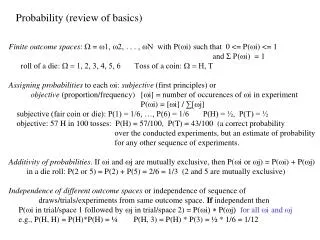
Probability (review of basics) Finite outcome spaces: = 1, 2, . . . , N with P(i) such that 0 <= P(i) <= 1 and Σ P(i) = 1 roll of a die: = 1, 2, 3, 4, 5, 6 Toss of a coin: = H, T Assigning probabilities to each i: subjective (first principles) or objective (proportion/frequency) [i] = number of occurences of i in experiment P(i) = [i] / ∑[j] subjective (fair coin or die): P(1) = 1/6, …, P(6) = 1/6 P(H) = ½, P(T) = ½ objective: 57 H in 100 tosses: P(H) = 57/100, P(T) = 43/100 (a correct probability over the conducted experiments, but an estimate of probability for any other sequence of experiments. Additivity of probabilities. If i and j are mutually exclusive, then P(i or j) = P(i) + P(j) in a die roll: P(2 or 5) = P(2) + P(5) = 2/6 = 1/3 (2 and 5 are mutually exclusive) Independence of different outcome spaces or independence of sequence of draws/trials/experiments from same outcome space. If independent then P(iin trial/space 1 followed by jin trial/space 2) = P(i) * P(j) for all iand j e.g., P(H, H) = P(H)*P(H) = ¼ P(H, 3) = P(H) * P(3) = ½ * 1/6 = 1/12
Countably infinite outcome spaces: e.g., flip a coin until first head • = H, TH, TTH, TTTH, ….. • P(H) = ½, P(TH) = ¼, P(TTH) = 1/8, P(TTTH) = 1/16, …. • probabilities must still sum to 1, since these outcomes are mutually exclusive. • ∑ 1/(2^(i+1)) = 1 • Joint outcome spaces and probabilities: W1 XW2 • if W1 = H, T then W1 XW1 = H,H H,T T,H T,T • (each with a probability, probabilities must sum to 1) • if W2 = 1, 2, 3, 4, 5, 6 then W1 XW2 = H,1 H,2 … H,6 T,1 ….. T,6 Random “variables”: a real-valued function defined over an outcome space: • = H, TH, TTH, TTTH, ….. • X1() = 0 1 2 3 …. (# of T before first H) • X2() 0.00001 ….. 0.0002 … (muscle fatigue) • X3() 100.0 …………95.4 ….. (patience) A random variable defines an outcome space. Probabilities can be assigned to random variable values. inf i=0
Expected value of a random variable: EX = ∑ [xi * P(X()=xi)] = ∑ [X(i )*P(i )] where xi is a value of the random “variable”X(), and i in an outcome in Expected number of examined nodes in successful search of a binary search tree 10 e.g., 4 15 • = (lookup) 10, 4, 15, 2, 11, 17, 14 P(i ) 0.1 0.1 0.05 0.05 0.2 0.3 0.2 X(i ) 1 2 2 3 3 3 4 EX = 1(0.1) + 2(0.1+0.05) + 3(0.05+0.2+0.3) + 4(0.2) 2 11 17 14 Random variables used to represent cost (space, time), value (goodness, utility), etc.
EX = ∑ [xi * P(X()=xi)] = ∑ [X(i )*P(i )] xi i Max node Expected minmax Chance node (Min rolls) 0.8 0.4 0.2 0.6 Min node Chance node (Max rolls) 0.5 0.5 1.0 0.3 0.8 0.7 1.0 0.3 1.0 1.0 0.7 0.2 B1 B2 B3 B4 B5 B6 B7 B8 B9 BA BB BC BD BE BF BG BH BI BJ BK BL BM BN i 5 2 3 4 2 8 1 6 3 2 4 4 9 3 1 7 4 3 1 2 8 6 6 X(i )
EX = ∑ [xi * P(X()=xi)] = ∑ [X(i )*P(i )] xi i Expected minmax 0.8 0.4 0.2 0.6 0.5 0.5 1.0 0.3 0.8 0.7 1.0 0.3 1.0 1.0 0.7 0.2 7 5 4 8 6 2 9 3 4 2 8 6 B1 B2 B3 B4 B5 B6 B7 B8 B9 BA BB BC BD BE BF BG BH BI BJ BK BL BM BN i 5 2 3 4 2 8 1 6 3 2 4 4 9 3 1 7 4 3 1 2 8 6 6 X(i )
EX = ∑ [xi * P(X()=xi)] = ∑ [X(i )*P(i )] xi i Expected minmax (0.7 * 2) + (0.3 * 9) 0.8 0.4 0.2 0.6 8 6 4.1 3 4.6 6.2 6 4.5 0.5 0.5 1.0 0.3 0.8 0.7 1.0 0.3 1.0 1.0 0.7 0.2 7 5 4 8 6 2 9 3 4 2 8 6 B1 B2 B3 B4 B5 B6 B7 B8 B9 BA BB BC BD BE BF BG BH BI BJ BK BL BM BN i 5 2 3 4 2 8 1 6 3 2 4 4 9 3 1 7 4 3 1 2 8 6 6 X(i )
EX = ∑ [xi * P(X()=xi)] = ∑ [X(i )*P(i )] xi i Expected minmax (0.2 * 4.5) + (0.8 * 4.1) 4.18 4.2 0.8 0.4 0.2 0.6 4.5 4.1 3 6 8 6 4.1 3 4.6 6.2 6 4.5 0.5 0.5 1.0 0.3 0.8 0.7 1.0 0.3 1.0 1.0 0.7 0.2 7 5 4 8 6 2 9 3 4 2 8 6 B1 B2 B3 B4 B5 B6 B7 B8 B9 BA BB BC BD BE BF BG BH BI BJ BK BL BM BN i 5 2 3 4 2 8 1 6 3 2 4 4 9 3 1 7 4 3 1 2 8 6 6 X(i )
Conditional probability: P(e1 | e2) = P(e1 and e2) / P(e2) where e1 is an event (a draw from an outcome space including the value of a random variable, and e2 is a draw from another outcome space or a proceeding/preceding draw from the same outcome space as e1 was drawn from. e.g., P(flu | sore-throat) = P(flu and sore-throat) / P(sore-throat) P(battery-dead | car-wont-start) = P(battery-dead and car-wont-start) / P(car-wont-start) In terms of objective probability assignment P(e1 | e2) = P(e1 and e2) / P(e2) = [[e1 and e2] / [o]] / [[e2] / [o]] = [e1 and e2] / [e2] where [o] = [e1 and e2] + [e1 and ~e2] + [~e1 + e2] + [~e1 + ~e2] = ([e1 and e2] + [e1 and ~e2]) + ([~e1 + e2] + [~e1 + ~e2]) = [e1] + [~e1] = ([e1 and e2] + [~e1 and e2]) + ([e1 + ~e2] + [~e1 + ~e2]) = [e2] + [~e2]
Bayes rule: • P(e1 | e2) = P(e1 and e2) / P(e2) P(e1|e2)P(e2) = P(e1 and e2) • P(e2 | e1) = P(e1 and e2) / P(e1) P(e2|e1)P(e1) = P(e1 and e2) • P(e1 | e2) = [P(e2 | e1) * P(e1)] / P(e2) Consider that a diagnosticianmay want to estimate P(Di | Sj) where Di is a disease, Sj is a symptom. P(Di | Sj) is hard for most experts to accurately estimate, but P(Di | Sj) = [P(Sj | Di) * P(Di)] / P(Sj) and P(Sj | Di) and P(Di) is easier for experts to accurately estimate. P(Sj) is hard to estimate, but it may not be important! P(D1 | Sj) = [P(Sj | D1) * P(D1)] / P(Sj) P(D2 | Sj) = [P(Sj | D2) * P(D2)] / P(Sj) which Di (disease) is most probable ….. note that P(Sj) is constant across choices P(DM | Sj) = [P(Sj | DM) * P(DM)] / P(Sj)
P(D1 | Sj) = [P(Sj | D1) * P(D1)] / P(Sj) P(D2 | Sj) = [P(Sj | D2) * P(D2)] / P(Sj) ….. P(DM | Sj) = [P(Sj | DM) * P(DM)] / P(Sj) P(D1 | Sj) a P(Sj | D1) * P(D1) P(D2 | Sj) a P(Sj | D2) * P(D2) answering which Di which is most probable ….. does not require P(Sj) P(DM | Sj) a P(Sj | DM) * P(DM) proportional to
Chain rule: Consider P(e1 and e2) = P(e1 | e2) P(e2) P(e1 and e2 and e3) = P(e1 | e2 and e3) P(e2 and e3) = P(e1 | e2 and e3) P(e2 | e3) P(e3) In general: P(e1, e2, e3, … , eN) read “,” as “and” = P(e1 | e2, e3, … , eN) P(e2 | e3, …., eN) P(e3 | e4,…,eN) …. P(e(N-1) | eN) P(eN) Put the chain rule and Bayes rule together: P(Di | S1, S2, …, SN) = [P(S1, S2, …, SN | Di) P(Di)] / P(S1, S2, … SN) = P(Di) * P(S1 | Di) * P(S2 | Di, S1) * … * P(SN | Di, S1,…,S(N-1)) P(S1) P(S2|S1) P(SN | S1,…, S(N-1)) a P(Di) * P(S1 | Di) * P(S2 | Di, S1) * … * P(SN | Di, S1,…,S(N-1)) allows Bayesian updating Bayes rule Chain rule
Where do P(Sj | Di, S1, S2, …, S(j-1)) come from??? Would need a lot of data for an objective assignment that was accurate Experts find it difficult to estimate in a subjective assignment Independence revisited Outcome spaces 1 and 2 are independent iff P(iand j) = P(i) * P(j) for all i in 1 and all j in 2 P(iand j) = P(i| j)P(j) = P(i) * P(j) P(i| j) = P(i) P(j| i) = P(j) Alternate definition of independence if independent
Conditional independence • 1 and 2 are conditionally independent given (any known outcome from) 3 iff • P(i and j | k ) = P(i | k ) * P(j | k ) for all i in 1, all j in 2 , and all k in 3 • P(i | j and k ) = P(i | k ) P(i and j | k ) = P(i | j and k ) P(j | k ) • P(j | i and k ) = P(j | k ) • We can also speak of 1 and 2 as conditionally independent given a particular • outcome from 3 • If symptoms independent given disease then • P(Di | S1, S2, …SN) • a • P(Di) * P(S1 | Di) * P(S2 | Di, S1) * … * P(SN | Di, S1,…,S(N-1)) • = • P(Di) * P(S1 | Di) * P(S2 | Di) * … * P(SN | Di)
Conditional expectation E(X | Y =yj) = ∑ xi P(X = xi | Y =yj) = ∑ X(i) P(W =i | Y =yj) xi i Si Si1 Si2 Si11 Si12 Si21 Si22 P(Si1 | Si, Op1) P(Si2 | Si, Op1) P(Si21 | Si2, Si, Op2) P(Si11 | Si, Op1 Si1, Op2) P(Si22 | Si, Op1, Si2, Op2) P(Si12 | Si, Op1, Si1, Op2) Ui21 Ui22 Ui11 Ui12 Assume a plan executer in an environment in which operators do not achieve their effects with certainty, but in which some Add/Del effects of an operator may not be in effect after an operator has been applied. Then, with some probablity, applying Op1 from state Si will lead to state Si1 and with some probability it will lead to Si2, etc. The U values are utility values of the possible resulting states (e.g., the number of goal conditions Satisfied by the state).
Conditional expectation E(X | Y =yj) = ∑ xi P(X = xi | Y =yj) = ∑ X(i) P(W =i | Y =yj) xi i Si Si1 Si2 Si11 Si12 Si21 Si22 P(Si1 | Si, Op1) P(Si2 | Si, Op1) P(Si21 | Si, Op1, Si2,Op2) P(Si11 | Si, Op1, Si1, Op2) P(Si12 | Si, Op1, Si1, Op2) P(Si22 | Si, Op1,Si2,Op2) Ui21 Ui22 Ui11 Ui12 EU(Si1 | Si, Op1) = P(Si11 | Si, Op1, Si1, Op2) * Uill + P(Si12 | Si, Op1, Si1, Op2) * Uil2
Conditional expectation E(X | Y =yj) = ∑ xi P(X = xi | Y =yj) = ∑ X(i) P(W =i | Y =yj) xi i EU(Si) = P(Si1 | Si, Op1) * EU(Si1 |Si, Op1) + P(Si2 | Si, Op1) * EU(Si2 |Si, Op1) Si Si1 Si2 Si11 Si12 Si21 Si22 P(Si1 | Si, Op1) P(Si2 | Si, Op1) P(Si21 | Si, Op1, Si2,Op2) P(Si11 | Si, Op1, Si1, Op2) P(Si12 | Si, Op1, Si1, Op2) P(Si22 | Si, Op1,Si2,Op2) Ui21 Ui22 Ui11 Ui12 EU(Si1 | Si, Op1) = P(Si11 | Si, Op1, Si1, Op2) * Uill + P(Si12 | Si, Op1, Si1, Op2) * Uil2