From PCA to Confirmatory FA
350 likes | 501 Views
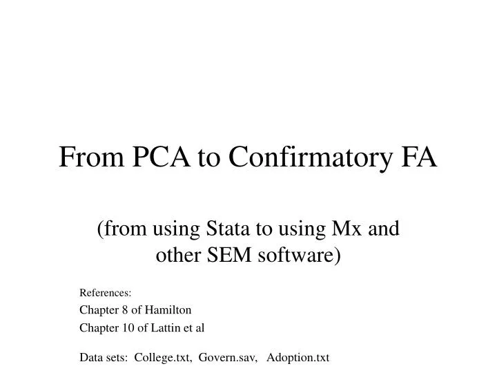
From PCA to Confirmatory FA. (from using Stata to using Mx and other SEM software) References: Chapter 8 of Hamilton Chapter 10 of Lattin et al Data sets: College.txt, Govern.sav, Adoption.txt. Class 1. Principal Components Exploratory Factor Model Confirmatory Factor Model.

From PCA to Confirmatory FA
E N D
Presentation Transcript
From PCA to Confirmatory FA (from using Stata to using Mx and other SEM software) References: Chapter 8 of Hamilton Chapter 10 of Lattin et al Data sets: College.txt, Govern.sav, Adoption.txt
Class 1 • Principal Components • Exploratory Factor Model • Confirmatory Factor Model
Principal Components Basic principles and the use of the method, with an example Chapter 8 of Hamilton, pp. 249-267
http://lib.stat.cmu.edu/DASL/Datafiles/Colleges.html data=read.table("G:/Albert/COURSES/RMMSS/Schools1.txt", header=T) names(data) [1] "School" "SchoolT" "SAT" "Accept" "CostSt" "Top10" "PhD" [8] "Grad" attach(data) pairs(data[,3:8]) lCost=log(CostSt) cdata=cbind(data[,3:4], lCost, data[,6:8]) pairs(cdata)
Principal Components Analysis (PCA) Yj = aj1PC1+ aj2PC2 + Ej, j = 1, 2, ... P the Yj are manifest variables Ej = aj3PC3 + .... ajp PCp the PC are called principal components Let Rj2 the R2 of the (linear) regression of Yj on PC1and PC2 In PCA, the a’s are choosen so to maximize sumj Rj2
use "G:\Albert\COURSES\RMMSS\school1.dta", clear . edit - preserve . summarize sat accept costst top10 phd grad Variable | Obs Mean Std. Dev. Min Max -------------+-------------------------------------------------------- sat | 50 1263.96 62.32959 1109 1400 accept | 50 37.84 13.36361 17 67 costst | 50 30247.2 15266.17 17520 102262 top10 | 50 74.44 13.51516 47 98 phd | 50 90.56 8.258972 58 100 -------------+-------------------------------------------------------- grad | 50 83.48 7.557237 61 95 .
Normalized pc . . gen lcost = log(costst) . pca sat accept lcost top10 phd grad, factors(2) (obs=50) (principal components; 2 components retained) Component Eigenvalue Difference Proportion Cumulative ------------------------------------------------------------------ 1 3.01940 1.74300 0.5032 0.5032 2 1.27640 0.52532 0.2127 0.7160 3 0.75108 0.25948 0.1252 0.8411 4 0.49160 0.25118 0.0819 0.9231 5 0.24042 0.01930 0.0401 0.9631 6 0.22112 . 0.0369 1.0000 Eigenvectors Variable | 1 2 -------------+--------------------- sat | 0.48705 -0.20272 accept | -0.47435 0.20082 lcost | 0.38708 0.30674 top10 | 0.45710 0.28373 phd | 0.27982 0.55460 grad | 0.31732 -0.66060 . greigen . score f1 f2 (based on unrotated principal components) Scoring Coefficients Variable | 1 2 -------------+--------------------- sat | 0.48705 -0.20272 accept | -0.47435 0.20082 lcost | 0.38708 0.30674 top10 | 0.45710 0.28373 phd | 0.27982 0.55460 grad | 0.31732 -0.66060 . . summarize f1 f2 Variable | Obs Mean Std. Dev. Min Max -------------+-------------------------------------------------------- f1 | 50 2.76e-09 1.737641 -2.693964 3.290203 f2 | 50 -7.38e-09 1.129777 -2.067842 3.50152
. cor sat accept lcost top10 phd grad f1 f2 (obs=50) | sat accept lcost top10 phd grad f1 f2 -------------+------------------------------------------------------------------------ sat | 1.0000 accept | -0.6068 1.0000 lcost | 0.5697 -0.2972 1.0000 top10 | 0.5093 -0.6163 0.5321 1.0000 phd | 0.2209 -0.3117 0.3155 0.4486 1.0000 grad | 0.5691 -0.5622 0.0999 0.1613 -0.0554 1.0000 f1 | 0.8463 -0.8243 0.6726 0.7943 0.4862 0.5514 1.0000 f2 | -0.2290 0.2269 0.3465 0.3206 0.6266 -0.7463 -0.0000 1.0000
library(mva) help('factanal') help('princomp') pca=princomp(cdata,cor=T, scores=T) biplot(pca) > summary(pca) Importance of components: Comp.1 Comp.2 Comp.3 Comp.4 Comp.5 Standard deviation 1.7376411 1.1297771 0.8666462 0.70114124 0.49032369 Proportion of Variance 0.5032328 0.2127327 0.1251793 0.08193317 0.04006955 Cumulative Proportion 0.5032328 0.7159655 0.8411447 0.92307790 0.96314745 round(cov(pca$scores[,1:2]),3) Comp.1 Comp.2 Comp.1 3.081 0.000 Comp.2 0.000 1.302
> data[,1] [1] Amherst Swarthmore Williams Bowdoin Wellesley [6] Pomona Wesleyan Middlebury Smith Davidson [11] Vassar Carleton ClarMcKenna Oberlin WashingtonLee [16] Grinnell MountHolyoke Colby Hamilton Bates [21] Haverford Colgate BrynMawr Occidental Barnard [26] Harvard Stanford Yale Princeton CalTech [31] MIT Duke Dartmouth Cornell Columbia [36] UofChicago Brown UPenn Berkeley JohnsHopkins [41] Rice UCLA UVa. Georgetown UNC [46] UMichican CarnegieMellon Northwestern WashingtonU UofRochester
DD=dist(pca$scores[,1:2], method ="euclidean", diag=FALSE) clust=hclust(DD, method="complete", members=NULL) plot(clust, labels=data[,1], cex=.8, col="blue", main="clustering of education")
Chapter 8 of Hamilton, pp. 270-281 (Exploratory) Factor Analysis Yj = aj1F1+ aj2F2 + Ej, j = 1, 2, ... P Ej = .... uncorrelated across j !! The a’s are choosen by principal factor method, ML, ... There is no unique solution (model is non-identified). Rotation methods to maximize interpretation (e.g., Varimax).
Exploratory Factor Analysis . factor sat accept lcost top10 phd grad, factors(3) ipf (obs=50) (iterated principal factors; 3 factors retained) Factor Eigenvalue Difference Proportion Cumulative ------------------------------------------------------------------ 1 2.75866 1.77477 0.6573 0.6573 2 0.98390 0.52915 0.2344 0.8917 3 0.45474 0.45357 0.1083 1.0000 4 0.00118 0.00100 0.0003 1.0003 5 0.00018 0.00160 0.0000 1.0003 6 -0.00142 . -0.0003 1.0000 Factor Loadings Variable | 1 2 3 Uniqueness -------------+------------------------------------------- sat | 0.80984 -0.12555 0.22792 0.27645 accept | -0.81206 0.20282 0.33555 0.18682 lcost | 0.65212 0.44139 0.42542 0.19894 top10 | 0.74504 0.32592 -0.23040 0.28561 phd | 0.38481 0.34884 -0.20905 0.68653 grad | 0.56121 -0.71011 0.11153 0.16835
Exploratory Factor Analysis > factanal(cdata, factors=2) Call: fac=factanal(cdata, factors=2, scores="regression") Uniquenesses: SAT Accept lCost Top10 PhD Grad 0.388 0.353 0.600 0.256 0.708 0.005 Loadings: Factor1 Factor2 SAT 0.484 0.615 Accept -0.523 -0.612 lCost 0.613 0.155 Top10 0.830 0.235 PhD 0.540 Grad 0.994 Factor1 Factor2 SS loadings 1.871 1.819 Proportion Var 0.312 0.303 Cumulative Var 0.312 0.615 Test of the hypothesis that 2 factors are sufficient. The chi square statistic is 11.47 on 4 degrees of freedom. The p-value is 0.0217 > > summary(fac) Length Class Mode converged 1 -none- logical loadings 12 loadings numeric uniquenesses 6 -none- numeric correlation 36 -none- numeric criteria 3 -none- numeric factors 1 -none- numeric dof 1 -none- numeric method 1 -none- character scores 100 -none- numeric STATISTIC 1 -none- numeric PVAL 1 -none- numeric n.obs 1 -none- numeric call 4 -none- call >
(Confirmatory) Factor Analysis Yj = aj1F1+ aj2F2 + Ej, j = 1, 2, ... P Ej = .... uncorrelated across j !! Some of the a’s are free, other restricted a priori (to 0s, 1s, or by equality among them), estimation method is ML, GLS,... There is uniqueness in the solution (an identified model).
Lattin and Roberts data of adoption new technologiesp. 366 of Lattin et al. See the data file adoption.txt in RMMRS
data=read.table("E:/Albert/COURSES/RMMSS/Mx/ADOPTION.txt", header=T) names(data) [1] "ADOPt1" "ADOPt2" "VALUE1" "VALUE2" "VALUE3" "USAGE1" "USAGE2" "USAGE3" attach(data) round(cov(data, use="complete.obs"),2) ADOPt1 ADOPt2 VALUE1 VALUE2 VALUE3 USAGE1 USAGE2 USAGE3 ADOPt1 675.17 489.24 6.25 5.46 4.08 10.62 11.69 7.12 ADOPt2 489.24 994.31 4.16 4.46 3.42 16.35 17.92 12.17 VALUE1 6.25 4.16 0.95 0.37 0.45 0.16 0.19 0.12 VALUE2 5.46 4.46 0.37 0.83 0.31 0.11 0.12 0.07 VALUE3 4.08 3.42 0.45 0.31 0.86 0.13 0.18 0.05 USAGE1 10.62 16.35 0.16 0.11 0.13 0.76 0.64 0.45 USAGE2 11.69 17.92 0.19 0.12 0.18 0.64 0.92 0.55 USAGE3 7.12 12.17 0.12 0.07 0.05 0.45 0.55 0.64 dim(data) [1] 188 8
Adoption.dat Data Nimput=8 Nobservations=188 CMatrix 675.17 489.24 994.31 6.25 4.16 0.95 5.46 4.46 0.37 0.83 4.08 3.42 0.45 0.31 0.86 10.62 16.35 0.16 0.11 0.13 0.76 11.69 17.92 0.19 0.12 0.18 0.64 0.92 7.12 12.17 0.12 0.07 0.05 0.45 0.55 0.64 Labels ADOPt1 ADOPt2 VALUE1 VALUE2 VALUE3 USAGE1 USAGE2 USAGE3
Exploratory Factor Analysis, ML method > data=read.table("E:/Albert/COURSES/RMMSS/Mx/ADOPTION.txt", header=T) > names(data) [1] "ADOPt1" "ADOPt2" "VALUE1" "VALUE2" "VALUE3" "USAGE1" "USAGE2" "USAGE3" attach(data) factanal(cbind(VALUE1, VALUE2,VALUE3,USAGE1, USAGE2,USAGE3), factors=2, rotation="varimax") Call: factanal(x = cbind(VALUE1, VALUE2, VALUE3, USAGE1, USAGE2, USAGE3), factors = 2) Uniquenesses: VALUE1 VALUE2 VALUE3 USAGE1 USAGE2 USAGE3 0.493 0.648 0.484 0.291 0.165 0.292 Loadings: Factor1 Factor2 VALUE1 0.127 0.700 VALUE2 0.586 VALUE3 0.714 USAGE1 0.823 0.179 USAGE2 0.896 0.179 USAGE3 0.836 Factor1 Factor2 SS loadings 2.209 1.418 Proportion Var 0.368 0.236 Cumulative Var 0.368 0.604 Test of the hypothesis that 2 factors are sufficient. The chi square statistic is 1.82 on 4 degrees of freedom. The p-value is 0.768
Adoption.dat Data Nimput=8 Nobservations=188 CMatrix 675.17 489.24 994.31 6.25 4.16 0.95 5.46 4.46 0.37 0.83 4.08 3.42 0.45 0.31 0.86 10.62 16.35 0.16 0.11 0.13 0.76 11.69 17.92 0.19 0.12 0.18 0.64 0.92 7.12 12.17 0.12 0.07 0.05 0.45 0.55 0.64 Labels ADOPt1 ADOPt2 VALUE1 VALUE2 VALUE3 USAGE1 USAGE2 USAGE3
Factor Analysis Charles Spearman, 1904 Acording to the two-factor theory of intelligence, the performance of any intellectual act requires some combination of "g", which is available to the same individual to the same degree for all intellectual acts, and of "specific factors" or "s" which are specific to that act and which varies in strength from one act to another. If one knows how a person performs on one task that is highly saturated with "g", one can safely predict a similar level of performance for a another highly "g" saturated task. Prediction of performance on tasks with high "s" factors are less accurate. Nevertheless, since "g" pervades all tasks, prediction will be significantly better than chance. Thus, the most important information to have about a person's intellectual ability is an estimate of their "g".
Spearman, 1904 Variables CLASSIC = V1 FRENCH = V2 ENGLISH = V3 MATH = V4 DISCRIM = V5 MUSIC = V6 Correlation matrix 1 .83 1 .78 .67 1 .70 .64 .64 1 .66 .65 .54 .45 1 .63 .57 .51 .51 .40 1 cases = 23;
Single-Factor Model * * * * * * V1 V2 V3 V4 V5 V6 * * * * * * F1
NT analysis RESIDUAL COVARIANCE MATRIX (S-SIGMA) : CLASSIC FRENCH ENGLISH MATH DISCRIM V 1 V 2 V 3 V 4 V 5 CLASSIC V 1 0.000 FRENCH V 2 -0.001 0.000 ENGLISH V 3 0.005 -0.029 0.000 MATH V 4 -0.006 0.003 0.046 0.000 DISCRIM V 5 -0.001 0.054 -0.015 -0.056 0.000 MUSIC V 6 0.003 0.005 -0.017 0.030 -0.049 MUSIC V 6 MUSIC V 6 0.000 CHI-SQUARE = 1.663 BASED ON 9 DEGREES OF FREEDOM PROBABILITY VALUE FOR THE CHI-SQUARE STATISTIC IS 0.99575 THE NORMAL THEORY RLS CHI-SQUARE FOR THIS ML SOLUTION IS 1.648 .
Loadings’ estimates, s.e. and z-test statistics CLASSIC =V1 = .960*F1 +1.000 E1 .160 6.019 FRENCH =V2 = .866*F1 +1.000 E2 .171 5.049 ENGLISH =V3 = .807*F1 +1.000 E3 .178 4.529 MATH =V4 = .736*F1 +1.000 E4 .186 3.964 DISCRIM =V5 = .688*F1 +1.000 E5 .190 3.621 MUSIC =V6 = .653*F1 +1.000 E6 .193 3.382
Estimates of unique-factors E1 -CLASSIC .078*I .064 I 1.224 I I E2 -FRENCH .251*I .093 I 2.695 I I E3 -ENGLISH .349*I .118 I 2.958 I I E4 - MATH .459*I .148 I 3.100 I I E5 -DISCRIM .527*I .167 I 3.155 I I E6 -MUSIC .574*I .180 I 3.184 I I
STANDARDIZED SOLUTION: CLASSIC =V1 = .960*F1 + .279 E1 FRENCH =V2 = .866*F1 + .501 E2 ENGLISH =V3 = .807*F1 + .591 E3 MATH =V4 = .736*F1 + .677 E4 DISCRIM =V5 = .688*F1 + .726 E5 MUSIC =V6 = .653*F1 + .758 E6
Data of Lawley and Maxwell GAELIC =V1 = .687*F1 + 1.000 E1 .076 9.079 ENGLISH =V2 = .672*F1 + 1.000 E2 .076 8.896 HISTO =V3 = .533*F1 + 1.000 E3 .076 7.047 ARITM =V4 = .766*F2 + 1.000 E4 .067 11.379 ALGEBRA =V5 = .768*F2 + 1.000 E5 .067 11.411 GEOMETRY=V6 = .616*F2 + 1.000 E6 .069 8.942 M0: /TITLE Lawley and Maxwell data /SPECIFICATIONS CAS=220; VAR=6; ME=ML; /LABEL v1 =Gaelic; v2 = English; v3 = Histo; v4 =aritm; v5 =Algebra; v6 =Geometry; /EQUATIONS V1= *F1 + E1; V2= *F1 + E2; V3= *F1 + E3; V4= *F1 + E4; V5= *F1 + E5; V6= *F1 + E6; /VARIANCES F1 = 1; E1 TO E6 = *; /COVARIANCES /MATRIX 1 .439 .410 .288 .329 .248 .439 1 .351 .354 .320 .329 .410 .351 1 .164 .190 .181 .288 .354 .164 1 .595 .470 .329 .320 .190 .595 1 .464 .248 .329 .181 .470 .464 1 /END M1: /EQUATIONS V1= *F1 + E1; V2= *F1 + E2; V3= *F1 + E3; V4= *F2 + E4; V5= *F2 + E5; V6= *F2 + E6; /VARIANCES F1 = 1; F2=1; E1 TO E6 = *; /COVARIANCES F1, F2 = *; COVARIANCES AMONG INDEPENDENT VARIABLES --------------------------------------- I F2 - F2 .597*I I F1 - F1 .072 I 8.308 M0, Single factor model CHI-SQUARE = 52.841, 9 df P-value LESS THAN 0.001 M1, Two factor model with correlated factors: CHI-SQUARE = 7.953, 8 df P-value = 0.43804