Download
1 / 39
390 likes | 499 Views
Green Cluster of Low-Power Embedded Hardware Server Accelerators. Presented by Navid Mohaghegh York University November 2011. Introduction. Internet is in every corner of our life Services on the internet are hosted on servers Powerful servers consume substantial amount of energy

E N D
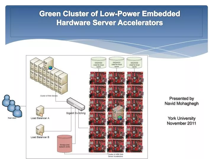
Green Cluster of Low-Power Embedded Hardware Server Accelerators Presented by Navid Mohaghegh York University November 2011
Introduction Internet is in every corner of our life Services on the internet are hosted on servers Powerful servers consume substantial amount of energy Google built one of their data centers in Oregon next to a power generation station It is desired to reduce the power consumption of data center without paying huge performance penalty
Power Consumption Power consumption is the largest operating expense in any server farm. An average powerful server uses around 450Watts every hour! Can the energy consumption be lowered?
Power Consumption TelTub Inc. is paying monthly fee of $275 CAD for each 15A circuit breaker and $850 for rental space and cooling of a standard rack mount (standard racks are 6.5 feet high with capacity of 10 4U servers per rack). Each 2MB/s bandwidth costs $50 CAD monthly. This will lead to a yearly cost of $20K for a standard rack ($120K if the average lifetime of a server is estimated to be 6 years).
Attempts to Reduce Power Consumption • Hard-Disk improvements • More efficient power supplies and coolers • More efficient CPUs with more cores • Use virtual machines • Prefetching and caching • Service differentiation • Using RAM for random access data intensive operations • Sleep modes vs. complete shutdown • Dynamic voltage scaling and throttling • Dynamic acceptance rate on peak traffic hours
Hard Disk Drive Improvements HDDs' mechanical and rotational nature force them to consume a substantial amount of energy. Average idle period for a server disk in a data center is very small compared to the time it takes to spin down and spin up the hard driver. Recently Solid State Drives that have absolutely no moving parts, are becoming more affordable and durable.
Attempts To Make More Efficient Power Supplies The increasing high-density servers may lead to a greater probability of thermal failure and hence require additional energy cost for cooling. An average 300 W server could easily consume 2.6 MWh of energy per year, with an additional 1 MWh for cooling. In this research, we are not focusing on ways to produce more efficient power supplies or thermodynamic techniques to produce more efficient chillers and cooling towers. We are focusing on the servers in particular and not the infrastructural parts of data centers.
Incerasse Core Per CPU Recently multi-core processors are becoming more affordable and popular. We even see commercial processors with 12 generic cores deployed in workstations. There have been attempts to use reconfigurable core architectures to provide a single chip solution to a broad range of targets. Concurrent I/O access will be an issue (e.g. cases like OpenMP, MPI)
Extensive Use of Virtual Machines Currently virtual machines are extensively usedin industry. There are less attempts to focus on bothpowerand performance optimization at the same time. Virtual machines running on the same physical server are tightly coupled and correlated to the underneath hardware and a simple state transition of any hardware component will affect the application performance of all the virtual machines. Solutions like PARTIC provide a two-layer control architecture that utilizes the CPU throttling while preserving the performance by maintaining load balancing among all virtual machines Using VM does not particularly improve the power consumption due to the overhead introduced by extra task switching caused by multiple virtual machines (push and pop).
Using Faster CPUs Currently, memory and I/O devices are not energy proportional. The key reason is that per-byte dynamic RAM power doesn’t scale as well as per-flop power from one generation of process technology to the next. This particularly proves that placing faster CPUs on servers to utilize more virtual machines does not necessarily decrease the power consumption drastically.
Prefetching and Service Differentiation In service differentiation customers (requests) are treated differently giving a priority for one type of requests (e.g. more important customers) over the others. In prefetching, data that is likely to be requested in the near future is prepared aheadof actually beingrequested. Both of these techniques can improve the performance of the system but there are no guarantees that a specific service level agreement (SLA) is met if no specific control system is applied. Less energyconsumption can be achieved in a non-direct manner as slow processors may be used
Using RAM for Random Access Data Intensive Operations Recently, Oracle introduced database servers that are mainly using RAM for their storage as a result of poor small file random access performance of the rotational disk based data centers Memory based clusters are very fast and also have a very highpower consumption and cost of ownership. (2GB DIMMs can consume as much as a 1 TB hard drive). SSDs are becoming more affordable and provide better random access response times compared to traditional HDDs.
Sleep Modes Instead of Complete Shutdown Servers can be put on sleep mode to consume less power during the less busy times. It is possible to build a mathematical model of solving an optimal power management (OPM). However, the situation will be a bit more complex once we are dealing with servers that are running multiple virtual machines.
Dynamic Voltage Scaling There has been efforts on various combination of dynamic voltage scaling and server throttling to reduce power consumption as it is not always optimal to run servers at their maximum power levels. Virtualization is becoming ubiquitous, and consequently diverse applications are increasingly sharing resources which drastically limit the ability to throttle hardware resources.
Dynamic Acceptance Rate on Peak Traffic Hours Using load balancing policies to distribute stateless requests (e.g. RESTful) among servers open the possibility to reach 10% energy savings (less context switch). Server over-utilization can be avoided by dynamically setting the maximum rate of accepted requests. Server resources can be protected from over-utilization by dynamically setting the acceptance rate of resource-intensive requests. Resource intensive requests and the resource they demand can be identified by their URL in the HTTP header. Identifying resource-intensive requests is not very easy (e.g. lengthy web-service calls)
High Performance Systems and Simple Tasks • Does an average web user care about super fast 15 ms response time or can they tolerate a little bit more (e.g 200 ms)? • Average network latency can vary widely (easily can reach 100ms). • May be simple tasks like web browsing don’t need very high performance servers. • Possibility of Embedded devices as servers or server accelerators • Lets conduct a simple experiments to do feasibility testing
Preliminarily Experiments • A lot of work is done in improving the performance of web servers and achieving a specific QoS. Earlier work in this area was mainly about service differentiation or using data prefetching. • Recently there have been attempts to use control theory and queuing systems to control the system and achieve QoS. • Common mistake is that guaranteeing the average response time does not necessarily yield to a specific SLA and QoS.
Preliminarily Experiments – PI Controller • is the average response time of all requests. ref is the required average response time. • 0 is the arrival rate (assumed to be Poisson arrival) • E[X] is the Expected value of the service time. • P0 is the admission probability in order to make =ref and p is the correction produced by the controller to p in order to guarantee the required ref. • Linearizing Eq. 1 using Taylor series around the operating point 0 we can solve for the PI controller • System is valid only in the steady state and for stable queues (by stable we mean average arrival rate is less than average service rate).
Preliminarily Experiments – On-demand Estimation of System Parameters • Estimating the System Parameters by monitoring the input and output of the server. • P is the admission probability • yis the system output • u is the system input • Z-1 is the delay operator. • ai and bi are system parameters estimated by measuring the output y and the input u • 0, 1, 0, 1, and K0 are chosen in order to achieve a reasonable overshot
Preliminarily Experiments – Additive Increase and Multiple Decrease • This idea came from the sliding window control in TCP . In TCP the window size is decreased (by a multiplicative factor) if there is a lost packet and is increased (by an additive factor) for successful transmission of a packet • If the queue size grows beyond a high threshold Nhigh the probability of accepting a new request is multiplied by , where 0<<1. • If the queue size drops below a low threshold Nlow, the admission probability is increased by , where 0<<1. The probability is bounded in the interval [0.1, 1] for practical purposes.
Preliminarily Experiments – Matlab Simulations • For all the experiments, we ran the simulation for 1600 s using Matlab. We collected the percentage of the requests accepted, the percentage of the requests that required less than 150 ms.and the average response time. For every experiment we considered two traffic scenarios: • Traffic A: We assumed an average exponential interarrival time of 55 ms and an average exponential service time of 35 ms. (64% utilization). The target response time is 150 ms. • Traffic B: We start as in Traffic A. At the simulation midpoint (after 800 s) we increase the arrival rate by decreasing the interarrival time to 45 ms (utilization of 78%). • The objective here is to see how the controller reacts to increasing the arrival rate in order to satisfy the QoS requirements.
Preliminarily Experiments – Matlab Simulations – PI controller Left figure shows a simulated run under traffic B. We can see that after 800 s the average response time increases. The main function of any controller is to adjust the admitting probability in order to avoid such a scenario Left figure shows the response time as a function of time. It is obvious that the controller suppressed the input in the second half of the simulation (after 800 s) leading to a more consistent (equal) response time.
Preliminarily Experiments – Matlab Simulations – On-demand Estimation of System Parameters Left figure shows a simulated run under traffic A while system control parameters calculated on-demand Left figure shows a simulated run under traffic B while system control parameters calculated on-demand
Preliminarily Experiments – Matlab Simulations – AIMD controller • Left figure shows a simulated run under traffic A while AIMD controller is used: • Nhigh=Ttarget/av, Nlow=Nhigh/2. • =0.4, and =0.8. • Where Ttarget is the target delay and is set to 150 ms and av is the average response time under traffic A Left figure shows a simulated run under traffic B while AIMD controller is used with above parameters.
Preliminarily Experiments – Matlab Simulations – Comparison of the Results
System Architecture We are using below software in this research: Linux as OS TFTP, PXE, NFS U-BOOT, INITRD, BusyBox LVS for high availability FastCGI, SNMP, Cherokee and PHP Admission Control and Load Balancing
Testing Results – Static Page Shortest and Average response-times Apache AB program is used to determine the shortest response-timeof a powerful server in contrast to proposed embedded cluster while the systems are not carrying heavy loads and serving a simple static page (a graphical image with file size of 2.1 kB) Result: response time of 1.1 ms and 4.3 ms respectively. Apache AB program is used to determine the average response-time of a powerful server in contrast to proposed embedded cluster while the systems are carrying heavy loads (cluster of laptops are generating 100 million requests of the exact same type with concurrency level of 300) and serving a simple static page (a graphical image with file size of 2.1 kB) Result: response time of 14.5 ms and 97.0 ms respectively. CPU Utilization was not high (less than 60%)
Testing Results – Dynamic Page Shortest and Average response-times Apache AB program is used to determine the shortest response-timeof a powerful server in contrast to proposed embedded cluster while the systems are not carrying heavy loads and serving a simple dynamic login page Result: response time of 1.0 ms and 7.6 ms respectively. Apache AB program is used to determine the average response-time of a powerful server in contrast to proposed embedded cluster while the systems are carrying heavy loads (cluster of laptops are generating 100 million requests of the exact same type with concurrency level of 300) and serving a simple dynamic login page Result: response time of 91.4 ms and 706.2ms respectively. CPU Utilization was not high (less than 60%)
Testing Results – Avoiding Exhaustion by Load Balancing and Admission Control
Testing Results – Avoiding Exhaustion by Load Balancing and Admission Control • Imagine a CPU intensive task (e.g. a simple iteration from 1 to 10,000) with deadline threshold of 2000 ms which is going to repeat 100,000 times. • If the concurrency is 10: • Cluster of four ARM 500 MHz will finish each job around an average of 85 ms • AMD 3.7 GHz with 6 cores will finish each job around an average of 7 ms • If the concurrency is 100: • Cluster of four ARM will finish each job around an average of 820 ms • AMD machine will finish each job around an average of 46 ms
Testing Results – Avoiding Exhaustion by Load Balancing and Admission Control • Imagine a CPU intensive task (e.g. a simple iteration from 1 to 10,000) with deadline threshold of 2000 ms which is going to repeat 100,000 times. • If the concurrency is 300: • Cluster of four ARM will finish each job around an average of 3629 ms • AMD machine will finish each job around an average of 730 ms • If concurrency is 1000: • Cluster of four ARM will halt eventually! • AMD machine will finish each job around an average of 3100 ms
Testing Results – Avoiding Exhaustion by Load Balancing and Admission Control • Now lets try to capture the system statistics every 500 ms and drop the requests: • If the concurrency is 300 with final drop rate of 20%: • Cluster of four ARM will finish each job around average of 1968 ms • AMD machine will finish each job around average of 381 ms • If concurrency is 1000 with final drop rate of 25%:: • Cluster of four ARM will halt eventually! finish the each job around 7900 ms • AMD machine will finish each job around average of 1803 ms • The most important result is that the system become stable. And at least we can avoid hitting the threshold while having 300 concurrent request hitting the ARM cluster.
Power Consumption Cluster of 4 ARM embedded machines running at 500 MHz did not use more than 25 Wh while pressured under heavy load (20,000 request/s) A single AMD 6-core machine running at 3.7 GHz used around 350 Whwhile pressured under heavy load (20,000 request/s) Results are based on: Blue Planet Electronic Energy Meter
Conclusion Reusable hardware Using low power embedded devices for simple tasks like application and database servers in web surfing A general embedded hardware is at least 4-7 times slower than an average powerful server but for most of the simple jobs, we do not care about instant computing power and all needed is the throughput and torque of the system. The fact that a page is loaded in 15 ms or loaded in 200 ms will not make a much difference for most of the Internet users.
Thank you! Questions?