Maximizing Program Efficiency: Dataflow Analysis & Optimization Techniques
Explore dataflow analysis, control flow graphs, reaching definitions, and safety concepts in program optimization. Learn how to apply constraints and formalize algorithms to enhance program efficiency.

Maximizing Program Efficiency: Dataflow Analysis & Optimization Techniques
E N D
Presentation Transcript
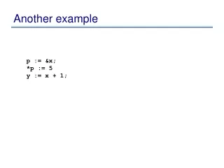
Another example p := &x; *p := 5 y := x + 1;
Another example p := &x; *p := 5 y := x + 1; x := 5; *p := 3 y := x + 1; ???
Another example for j := 1 to N for i := 1 to M a[i] := a[i] + b[j]
Another example for j := 1 to N for i := 1 to M a[i] := a[i] + b[j]
Another example area(h,w) { return h * w } h := ...; w := 4; a := area(h,w)
Another example area(h,w) { return h * w } h := ...; w := 4; a := area(h,w)
Optimization themes • Don’t compute if you don’t have to • unused assignment elimination • Compute at compile-time if possible • constant folding, loop unrolling, inlining • Compute it as few times as possible • CSE, PRE, PDE, loop invariant code motion • Compute it as cheaply as possible • strength reduction • Enable other optimizations • constant and copy prop, pointer analysis • Compute it with as little code space as possible • unreachable code elimination
Dataflow analysis: what is it? • A common framework for expressing algorithms that compute information about a program • Why is such a framework useful?
Dataflow analysis: what is it? • A common framework for expressing algorithms that compute information about a program • Why is such a framework useful? • Provides a common language, which makes it easier to: • communicate your analysis to others • compare analyses • adapt techniques from one analysis to another • reuse implementations (eg: dataflow analysis frameworks)
Control Flow Graphs • For now, we will use a Control Flow Graph representation of programs • each statement becomes a node • edges between nodes represent control flow • Later we will see other program representations • variations on the CFG (eg CFG with basic blocks) • other graph based representations
Example CFG x := ... y := ... x := ... y := ... y := ... p := ... if (...) { ... x ... x := ... ... y ... } else { ... x ... x := ... *p := ... } ... x ... ... y ... y := ... y := ... p := ... if (...) ... x ... ... x ... x := ... x := ... ... y ... *p := ... ... x ... ... x ... y := ...
An example DFA: reaching definitions • For each use of a variable, determine what assignments could have set the value being read from the variable • Information useful for: • performing constant and copy prop • detecting references to undefined variables • presenting “def/use chains” to the programmer • building other representations, like the DFG • Let’s try this out on an example
x := ... Visual sugar y := ... 1: x := ... 2: y := ... 3: y := ... 4: p := ... y := ... p := ... if (...) ... x ... 5: x := ... ... y ... ... x ... 6: x := ... 7: *p := ... ... x ... ... x ... x := ... x := ... ... y ... *p := ... ... x ... ... y ... 8: y := ... ... x ... ... x ... y := ...
1: x := ... 2: y := ... 3: y := ... 4: p := ... ... x ... 5: x := ... ... y ... ... x ... 6: x := ... 7: *p := ... ... x ... ... y ... 8: y := ...
1: x := ... 2: y := ... 3: y := ... 4: p := ... ... x ... 5: x := ... ... y ... ... x ... 6: x := ... 7: *p := ... ... x ... ... y ... 8: y := ...
Safety • When is computed info safe? • Recall intended use of this info: • performing constant and copy prop • detecting references to undefined variables • presenting “def/use chains” to the programmer • building other representations, like the DFG • Safety: • can have more bindings than the “true” answer, but can’t miss any
Reaching definitions generalized • DFA framework is geared towards computing information at each program point (edge) in the CFG • So generalize the reaching definitions problem by stating what should be computed at each program point • For each program point in the CFG, compute the set of definitions (statements) that may reach that point • Notion of safety remains the same
Reaching definitions generalized • Computed information at a program point is a set of var ! stmt bindings • eg: { x ! s1, x ! s2, y ! s3 } • How do we get the previous info we wanted? • if a var x is used in a stmt whose incoming info is in, then:
Reaching definitions generalized • Computed information at a program point is a set of var ! stmt bindings • eg: { x ! s1, x ! s2, y ! s3 } • How do we get the previous info we wanted? • if a var x is used in a stmt whose incoming info is in, then: { s | (x!s) 2in } • This is a common pattern • generalize the problem to define what information should be computed at each program point • use the computed information at the program points to get the original info we wanted
1: x := ... 2: y := ... 3: y := ... 4: p := ... ... x ... 5: x := ... ... y ... ... x ... 6: x := ... 7: *p := ... ... x ... ... y ... 8: y := ...
1: x := ... 2: y := ... 3: y := ... 4: p := ... ... x ... 5: x := ... ... y ... ... x ... 6: x := ... 7: *p := ... ... x ... ... y ... 8: y := ...
Using constraints to formalize DFA • Now that we’ve gone through some examples, let’s try to precisely express the algorithms for computing dataflow information • We’ll model DFA as solving a system of constraints • Each node in the CFG will impose constraints relating information at predecessor and successor points • Solution to constraints is result of analysis
Constraints for reaching definitions in s: x := ... out in s: *p := ... out
Constraints for reaching definitions • Using may-point-to information: out = in [ { x ! s | x 2 may-point-to(p) } • Using must-point-to aswell: out = in – { x ! s’ | x 2 must-point-to(p) Æ s’ 2 stmts } [ { x ! s | x 2 may-point-to(p) } in out = in – { x ! s’ | s’ 2 stmts } [ { x ! s } s: x := ... out in s: *p := ... out
Constraints for reaching definitions in s: if (...) out[0] out[1] in[0] in[1] merge out
Constraints for reaching definitions in out [ 0] = in Æ out [ 1] = in s: if (...) out[0] out[1] more generally: 8i . out [ i ] = in in[0] in[1] out = in [ 0] [in [ 1] merge more generally: out = iin [ i ] out
Flow functions • The constraint for a statement kind s often have the form: out = Fs(in) • Fs is called a flow function • other names for it: dataflow function, transfer function • Given information in before statement s, Fs(in) returns information after statement s • Other formulations have the statement s as an explicit parameter to F: given a statement s and some information in, F(s,in) returns the outgoing information after statement s
Flow functions, some issues • Issue: what does one do when there are multiple input edges to a node? • Issue: what does one do when there are multiple outgoing edges to a node?
Flow functions, some issues • Issue: what does one do when there are multiple input edges to a node? • the flow functions takes as input a tuple of values, one value for each incoming edge • Issue: what does one do when there are multiple outgoing edges to a node? • the flow function returns a tuple of values, one value for each outgoing edge • can also have one flow function per outgoing edge
Flow functions • Flow functions are a central component of a dataflow analysis • They state constraints on the information flowing into and out of a statement • This version of the flow functions is local • it applies to a particular statement kind • we’ll see global flow functions shortly...
Summary of flow functions • Flow functions: Given information in before statement s, Fs(in) returns information after statement s • Flow functions are a central component of a dataflow analysis • They state constraints on the information flowing into and out of a statement
d0 Back to example 1: x := ... 2: y := ... 3: y := ... 4: p := ... if(...) d1 = Fa(d0) d1 d2 = Fb(d1) d2 d3 = Fc(d2) d3 d4 = Fd(d3) d4 d9 = Ff(d5) d5 = Fe(d4) d9 d5 d10 = Fj(d9) d6 = Fg(d5) ... x ... 5: x := ... ... y ... ... x ... 6: x := ... 7: *p := ... d6 d10 d11 = Fk(d10) d7 = Fh(d6) d7 d11 d12 = Fl(d11) d8 = Fi(d7) d12 d8 d13 = Fm(d12, d8) merge ... x ... ... y ... 8: y := ... d13 How to find solutions for di? d14 = Fn(d13) d14 d15 = Fo(d14) d15 d16 = Fp(d15) d16
How to find solutions for di? • This is a forward problem • given information flowing in to a node, can determine using the flow function the info flow out of the node • To solve, simply propagate information forward through the control flow graph, using the flow functions • What are the problems with this approach?
d0 First problem 1: x := ... 2: y := ... 3: y := ... 4: p := ... if(...) d1 = Fa(d0) d1 d2 = Fb(d1) d2 d3 = Fc(d2) d3 d4 = Fd(d3) d4 d9 = Ff(d5) d5 = Fe(d4) d9 d5 d10 = Fj(d9) d6 = Fg(d5) ... x ... 5: x := ... ... y ... ... x ... 6: x := ... 7: *p := ... d6 d10 d11 = Fk(d10) d7 = Fh(d6) d7 d11 d12 = Fl(d11) d8 = Fi(d7) d12 d8 d13 = Fm(d12, d8) merge ... x ... ... y ... 8: y := ... d13 What about the incoming information? d14 = Fn(d13) d14 d15 = Fo(d14) d15 d16 = Fp(d15) d16
First problem • What about the incoming information? • d0 is not constrained • so where do we start? • Need to constrain d0 • Two options: • explicitly state entry information • have an entry node whose flow function sets the information on entry (doesn’t matter if entry node has an incoming edge, its flow function ignores any input)
Entry node out = { x ! s | x 2 Formals } s: entry out
d0 = Fentry() d0 Second problem 1: x := ... 2: y := ... 3: y := ... 4: p := ... if(...) d1 = Fa(d0) d1 d2 = Fb(d1) d2 d3 = Fc(d2) d3 d4 = Fd(d3) d4 d9 = Ff(d5) d5 = Fe(d4) d9 d5 d10 = Fj(d9) d6 = Fg(d5) ... x ... 5: x := ... ... y ... ... x ... 6: x := ... 7: *p := ... d6 d10 d11 = Fk(d10) d7 = Fh(d6) d7 d11 d12 = Fl(d11) d8 = Fi(d7) d12 d8 d13 = Fm(d12, d8) Which order to process nodes in? merge ... x ... ... y ... 8: y := ... d13 d14 = Fn(d13) d14 d15 = Fo(d14) d15 d16 = Fp(d15) d16
Second problem • Which order to process nodes in? • Sort nodes in topological order • each node appears in the order after all of its predecessors • Just run the flow functions for each of the nodes in the topological order • What’s the problem now?
Second problem, prime • When there are loops, there is no topological order! • What to do? • Let’s try and see what we can do
1: x := ... 2: y := ... 3: y := ... 4: p := ... ... x ... 5: x := ... ... y ... ... x ... 6: x := ... 7: *p := ... ... x ... ... y ... 8: y := ...
1: x := ... 2: y := ... 3: y := ... 4: p := ... ... x ... 5: x := ... ... y ... ... x ... 6: x := ... 7: *p := ... ... x ... ... y ... 8: y := ...