Download
1 / 1
10 likes | 106 Views
X-ray Line Profile Diagnostics of Shock Heated Stellar Winds Roban H. Kramer 1,2 , Stephanie K. Tonnesen 1 , David H. Cohen 1,2 , Stanley P. Owocki 3 , Asif ud-Doula 3 (1) Swarthmore College, (2) Prism Computational Sciences, (3) Bartol Research Institute, University of Delaware. for .

E N D
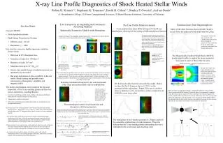
X-ray Line Profile Diagnostics of Shock Heated Stellar Winds Roban H. Kramer1,2, Stephanie K. Tonnesen1, David H. Cohen1,2, Stanley P. Owocki3, Asif ud-Doula3 (1) Swarthmore College, (2) Prism Computational Sciences, (3) Bartol Research Institute, University of Delaware for Line Transport in an Expanding and Continuum-Absorbing Medium Spherically Symmetric Models with Absorption The Line Profile Model is General It can parameterize many different types of wind X-ray distributions, allowing for the testing of different physical theories Emission Lines from Magnetospheres Hot Star Winds Many of the other hot stars observed with Chandra are not fit by the spherical wind model that fits z Pup • Chandra HETGS • Nested parabolic mirrors • High Energy Transmission Grating: • Effective area ~ 10 cm2 • Resolution ≤ ~ 1000 • Hot stars have massive, highly supersonic radiation driven winds: • Observed in UV absorption lines • Velocities of order few 1000 km s-1 • Densities of order 1010 cm-3 • Mass-loss rates up to 10-5 Msun yr-1 • Steady-state models based on radiation pressure are quantitatively successful • But many indications of time-variability in hot star winds: Shock heating and possibly some connection to photospheric variability and magnetic fields • The heating mechanisms, not to mention the physical properties, of the X-ray emitting plasma on these hot stars is not known. Leading theories: • Line force instability generated shocks, leading to hot plasma distributed throughout the wind (described by a filling factor), • Magnetically confined wind shocks, • Solar-type coronal magnetic heating (but hot stars are not thought to have dynamos and coronae). • In all cases, the X-ray emitting plasma is thermal and optically thin, emitting photons in lines. Especially in case (1) there is a bulk, cold wind component (which leads to the UV absorption lines) that is a source of X-ray continuum opacity. • - The speed of these winds has the potential to produce substantial Doppler broadening of the lines, while the continuum absorption can alter the line shapes through the spatial dependence of the absorption coupled with the spatial dependence of the Doppler shift in an organized flow. • - High-resolution X-ray spectroscopy of astrophysical objects has only in the last two years become feasible, and hot stars are one of the very few types of sources for which telescopes like Chandra can resolve X-ray line shapes. • - We can use the observed line shapes to infer the spatial- and velocity-distributions of the X-ray emitting plasma on hot stars, and thereby constrain models of X-ray production and wind dynamics. Varying the minimum radius of X-ray emission (R0) and the intrinsic optical depth of the wind () affects the shape of the profiles. Larger minimum radii exclude inner, slow-moving regions of the wind, resulting in broader, flatter profiles. Higher intrinsic optical depths obscure reddened regions, skewing the line blueward. Far left are contours of optical depth unity for different values of overlaying color velocity maps. Next to them are the corresponding line profiles. The majority of other hot stars observed with Chandra show line profiles that are broad but symmetric. They cannot be fit by any spherically symmetric wind model that includes absorption. Doppler shifting of the expanding wind broadens lines. To the observer on the left, the front of the wind is blueshifted and the back is redshifted. R0 = 1.5 R =1, q=1/2 To mimic a coronal model of X-ray production we let the emissivity drop off like a high power of 1/r, producing narrow profiles (below). The Magnetically Confined Wind Shock (MCWS) model might be able to explain the more symmetric lines seen in some of these other hot stars R0 = 3 R MHD simulations of magnetic wind shock scenario Thin, expanding, spherical shells produce flat-topped line profiles broadened by the shell velocity. Inner shells are slower and more dense, giving narrower, taller profiles. Occultation by the star removes light from the red edge of the profile. A continuous wind is built by integrating over shells from some minimum radius. A series of shells, added together, produce a stepped profile. Strong (~kG) large-scale dipole fields have been detected in some hot stars. A strong wind in the presence of such a field will be channeled toward the magnetic equator, where a standing shock will develop, heating the wind to many 106 K. R0 = 10 R The wind is depicted spatially in the color plots, with the hue indicating velocity with respect to an observer on the left, and the brightness of the ink indicating emissivity (scaling as density squared). Note the color scale above the third panel. Under each image is the resulting line profile with the bluest wavelengths (expressed in velocity units) on the left, and the reddest on the right. =1, q=1/2 Including continuum absorption by the cold component of the wind also preferentially removes red photons. We fit Chandra data from hot stars with this model. Below we show the Ne X Lyman-a line at 12.132 Å in the prototypical blue supergiant z Puppis. This star is a million times as luminous as the sun and has a surface temperature of 42000 K (seven times solar). (ud-Doula & Owocki 2002) At far left, contours of constant optical depth (integrated along the observer’s line of sight) are overlay a velocity color map. The resulting line profile (immediate left) shows the effect of an optically thick wind. We have begun to model axisymmetric, equatorially enhanced x-ray emitting flows, based on the MCWS model. The model below is a rotationally symmetric wind that emits only in a region 20o above and below the rotational equator. We model a radial outflow described by velocity and density laws. The viewing angle affects the appearance of the line profile. As is increases, both the doppler shift of the photons from the disk and the amount of occultation from the star also increase, affecting the line shape and the degree of asymmetry in the profile. Phenomenological model of wind emission and absorption with four parameters. 90o Schematic made by Dave Caption Analysis We have developed a physically meaningful line-profile model, yet one that is simple and not tied to any one proposed mechanism of hot-star X-ray production. Described in Owocki & Cohen (2001, ApJ, 559, 1108), the model assumes a smoothly and spherically symmetrically distributed accelerating X-ray emitting plasma subject to continuum attenuation by the cold stellar wind. All the emission physics is hidden in the emissivity, h. Note that spherical coordinates (m,r) are natural for the symmetry of the wind emission. The strong lines in the Chandra spectrum of z Puppis can be fit by reasonable combinations of wind parameters. These fits indicate that the X-ray emitting plasma surrounding this star is embedded in the accelerating and absorbing wind. The velocity is assumed to be of the form v(r)=v∞(1-R/r)b With the observer looking at the star and wind from one side, cylindrical coordinates (p,z) are more natural. 45o 0o where andbparameterize the absorption. And q and Ro parameterize the radial X-ray filling factor, thus the emissivity. It is this delta function that allows us to map m,r into wavelength, l. We solve these equations numerically with Mathematica.